


Supervised Learning Part I:Liner Regression
KeyWords:feature,hypothesis,cost
Main methods to actualize: CostFunction,GradientDescent,NormalEquation
To the features such as x1,x2 we have a hypothesis:  or in vector:
and to use this function,we have to define theta0,theta1.......We want to find these parameter which can fit the reality in maximum degree.So we set a new function called COST FUNCTION to describe the
difference between our hypothesis and the reality.
The cost function is  So what we do next is to find a theta which leads to Function J to have the minimum value.Now the Question is how to get the minimum value?Two methods are given:First is Gradient Descent.Second is Normal Equation.Both of them can get the minimum value of J and find the Theta.
So what we do next is to find a theta which leads to Function J to have the minimum value.Now the Question is how to get the minimum value?Two methods are given:First is Gradient Descent.Second is Normal Equation.Both of them can get the minimum value of J and find the Theta.
Gradient Descent:
To have a good a command of Gradient Descent,let's say something else.
You have to be familiar with the following mathematical formula :
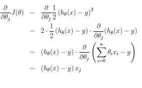
After you have known this,we can go on now!
Use formula 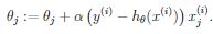 to update theta. If you have more than one feature,you need a loop to deal with it.In every loop,do
 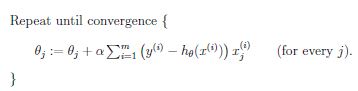 So in detail,the whole process looks like that:
to update theta. If you have more than one feature,you need a loop to deal with it.In every loop,do So in detail,the whole process looks like that:
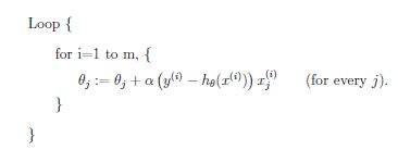
NOTICE I: in all above formula,there is a variable alpha(a) which is called learning rate.Alpha doesn't have a actual value, we often set it to 0.01 or 0.1.If alpha is too big, the loop will finish too quickly,so we may not have the proper answer,if too small,it will cost us a lot of time to run the program.
NOTICE II:when you have more than two features, you have to update theta simultaneously!!!
Normal Equation:
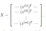
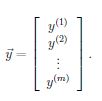
In another way,we can write X,Y into matrix style:
So 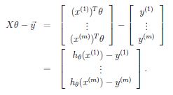
and the cost function is :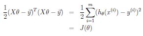
we can solve the equation and theta is :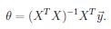
Apparently,we have have 10,000 or more dataset,Gradient descent is more efficient than normal equation.
Implement:
Liner Regression with one feature.
Main
%% Initialization
clear ; close all; clc

%% ==================== Part 1: Basic Function ====================
% Complete warmUpExercise.m
fprintf('Running warmUpExercise ... \n');
fprintf('5x5 Identity Matrix: \n');
warmUpExercise()

fprintf('Program paused. Press enter to continue.\n');
pause;


%% ======================= Part 2: Plotting =======================
fprintf('Plotting Data ...\n')
data = load('ex1data1.txt');
X = data(:, 1); y = data(:, 2);
m = length(y); % number of training examples

% Plot Data
% Note: You have to complete the code in plotData.m
plotData(X, y);

fprintf('Program paused. Press enter to continue.\n');
pause;

%% =================== Part 3: Gradient descent ===================
fprintf('Running Gradient Descent ...\n')

X = [ones(m, 1), data(:,1)]; % Add a column of ones to x
theta = zeros(2, 1); % initialize fitting parameters

% Some gradient descent settings
iterations = 1500;
alpha = 0.01;

% compute and display initial cost
computeCost(X, y, theta)

% run gradient descent
theta = gradientDescent(X, y, theta, alpha, iterations);

% print theta to screen
fprintf('Theta found by gradient descent: ');
fprintf('%f %f \n', theta(1), theta(2));

% Plot the linear fit
hold on; % keep previous plot visible
plot(X(:,2), X*theta, '-')
legend('Training data', 'Linear regression')
hold off % don't overlay any more plots on this figure

% Predict values for population sizes of 35,000 and 70,000
predict1 = [1, 3.5] *theta;
fprintf('For population = 35,000, we predict a profit of %f\n',...
    predict1*10000);
predict2 = [1, 7] * theta;
fprintf('For population = 70,000, we predict a profit of %f\n',...
    predict2*10000);

fprintf('Program paused. Press enter to continue.\n');
pause;

%% ============= Part 4: Visualizing J(theta_0, theta_1) =============
fprintf('Visualizing J(theta_0, theta_1) ...\n')

% Grid over which we will calculate J
theta0_vals = linspace(-10, 10, 100);
theta1_vals = linspace(-1, 4, 100);

% initialize J_vals to a matrix of 0's
J_vals = zeros(length(theta0_vals), length(theta1_vals));

% Fill out J_vals
for i = 1:length(theta0_vals)
    for j = 1:length(theta1_vals)
    t = [theta0_vals(i); theta1_vals(j)];
    J_vals(i,j) = computeCost(X, y, t);
    end
end


% Because of the way meshgrids work in the surf command, we need to
% transpose J_vals before calling surf, or else the axes will be flipped
J_vals = J_vals';
% Surface plot
figure;
surf(theta0_vals, theta1_vals, J_vals)
xlabel('\theta_0'); ylabel('\theta_1');

% Contour plot
figure;
% Plot J_vals as 15 contours spaced logarithmically between 0.01 and 100
contour(theta0_vals, theta1_vals, J_vals, logspace(-2, 3, 20))
xlabel('\theta_0'); ylabel('\theta_1');
hold on;
plot(theta(1), theta(2), 'rx', 'MarkerSize', 10, 'LineWidth', 2);
ComputeCost:
function J = computeCost(X, y, theta)
%COMPUTECOST Compute cost for linear regression
%   J = COMPUTECOST(X, y, theta) computes the cost of using theta as the
%   parameter for linear regression to fit the data points in X and y

% Initialize some useful values
m = length(y); % number of training examples

% You need to return the following variables correctly
J = 0;

% ====================== YOUR CODE HERE ======================
% Instructions: Compute the cost of a particular choice of theta
%               You should set J to the cost.

J = 1/(2 * m) * (X * theta - y)' * (X * theta - y);

% =========================================================================

end
Gradient Descent:
function [theta, J_history] = gradientDescent(X, y, theta, alpha, num_iters)
%GRADIENTDESCENT Performs gradient descent to learn theta
%   theta = GRADIENTDESENT(X, y, theta, alpha, num_iters) updates theta by
%   taking num_iters gradient steps with learning rate alpha

% Initialize some useful values
m = length(y); % number of training examples
J_history = zeros(num_iters, 1);

for iter = 1:num_iters

    % ====================== YOUR CODE HERE ======================
    % Instructions: Perform a single gradient step on the parameter vector
    %               theta.
    %
    % Hint: While debugging, it can be useful to print out the values
    %       of the cost function (computeCost) and gradient here.
    %
    % Batch gradient descent
    Update = 0;
    for i = 1:m
        Update = Update + alpha/m * (y(i) - X(i,:) * theta) * X(i, :)';
    end
    theta = theta + Update;

    % ============================================================

    % Save the cost J in every iteration
    J_history(iter) = computeCost(X, y, theta);

end

end
Running process:
Running Gradient Descent ...

ans =

   32.0727

Theta found by gradient descent: -3.630291 1.166362
For population = 35,000, we predict a profit of 4519.767868
For population = 70,000, we predict a profit of 45342.450129
Program paused. Press enter to continue.
Visualizing J(theta_0, theta_1) ...
Liner Regression with mutli feature:
Main:
%% Initialization

%% ================ Part 1: Feature Normalization ================

%% Clear and Close Figures
clear ; close all; clc

fprintf('Loading data ...\n');

%% Load Data
data = load('ex1data2.txt');
X = data(:, 1:2);
y = data(:, 3);
m = length(y);

% Print out some data points
fprintf('First 10 examples from the dataset: \n');
fprintf(' x = [%.0f %.0f], y = %.0f \n', [X(1:10,:) y(1:10,:)]');

fprintf('Program paused. Press enter to continue.\n');
pause;

% Scale features and set them to zero mean
fprintf('Normalizing Features ...\n');

[X mu sigma] = featureNormalize(X);

% Add intercept term to X
X = [ones(m, 1) X];


%% ================ Part 2: Gradient Descent ================

% ====================== YOUR CODE HERE ======================
% Instructions: We have provided you with the following starter
%               code that runs gradient descent with a particular
%               learning rate (alpha).
%
%               Your task is to first make sure that your functions -
%               computeCost and gradientDescent already work with
%               this starter code and support multiple variables.
%
%               After that, try running gradient descent with
%               different values of alpha and see which one gives
%               you the best result.
%
%               Finally, you should complete the code at the end
%               to predict the price of a 1650 sq-ft, 3 br house.
%
% Hint: By using the 'hold on' command, you can plot multiple
%       graphs on the same figure.
%
% Hint: At prediction, make sure you do the same feature normalization.
%

fprintf('Running gradient descent ...\n');

% Choose some alpha value
alpha = 0.01;
num_iters = 1000;

% Init Theta and Run Gradient Descent
theta = zeros(3, 1);
[theta, J_history] = gradientDescentMulti(X, y, theta, alpha, num_iters);

% Plot the convergence graph
figure;
plot(1:numel(J_history), J_history, '-b', 'LineWidth', 2);
xlabel('Number of iterations');
ylabel('Cost J');

% Display gradient descent's result
fprintf('Theta computed from gradient descent: \n');
fprintf(' %f \n', theta);
fprintf('\n');

% Estimate the price of a 1650 sq-ft, 3 br house
% ====================== YOUR CODE HERE ======================
% Recall that the first column of X is all-ones. Thus, it does
% not need to be normalized.
x_predict = [1 1650 3];
for i=2:3
    x_predict(i) = (x_predict(i) - mu(i-1)) / sigma(i-1);
end
price = x_predict * theta;

% ============================================================

fprintf(['Predicted price of a 1650 sq-ft, 3 br house ' ...
         '(using gradient descent):\n $%f\n'], price);

fprintf('Program paused. Press enter to continue.\n');
pause;

%% ================ Part 3: Normal Equations ================

fprintf('Solving with normal equations...\n');

% ====================== YOUR CODE HERE ======================
% Instructions: The following code computes the closed form
%               solution for linear regression using the normal
%               equations. You should complete the code in
%               normalEqn.m
%
%               After doing so, you should complete this code
%               to predict the price of a 1650 sq-ft, 3 br house.
%

%% Load Data
data = csvread('ex1data2.txt');
X = data(:, 1:2);
y = data(:, 3);
m = length(y);

% Add intercept term to X
X = [ones(m, 1) X];

% Calculate the parameters from the normal equation
theta = normalEqn(X, y);

% Display normal equation's result
fprintf('Theta computed from the normal equations: \n');
fprintf(' %f \n', theta);
fprintf('\n');


% Estimate the price of a 1650 sq-ft, 3 br house
% ====================== YOUR CODE HERE ======================
x_predict = [1 1650 3];
price = x_predict * theta;
% ============================================================

fprintf(['Predicted price of a 1650 sq-ft, 3 br house ' ...
         '(using normal equations):\n $%f\n'], price);
Normal Equations:
function [theta] = normalEqn(X, y)
%NORMALEQN Computes the closed-form solution to linear regression
%   NORMALEQN(X,y) computes the closed-form solution to linear
%   regression using the normal equations.

theta = zeros(size(X, 2), 1);

% ====================== YOUR CODE HERE ======================
% Instructions: Complete the code to compute the closed form solution
%               to linear regression and put the result in theta.
%
theta = inv(X'* X)*X'*y;
% ============================================================

end
Result:
Normalizing Features ...
Running gradient descent ...
Theta computed from gradient descent:
 340397.963535
 109848.008460
 -5866.454085

Predicted price of a 1650 sq-ft, 3 br house (using gradient descent):
 $293237.161479
Program paused. Press enter to continue.
Solving with normal equations...
Theta computed from the normal equations:
 89597.909543
 139.210674
 -8738.019112

Predicted price of a 1650 sq-ft, 3 br house (using normal equations):
 $293081.464335


 1304
1304


 被折叠的 条评论
为什么被折叠?
被折叠的 条评论
为什么被折叠?
 到【灌水乐园】发言


