


这篇文章主要是最近整理《数据挖掘与分析》课程中的作品及课件过程中,收集了几段比较好的代码供大家学习。同时,做数据分析到后面,除非是研究算法创新的,否则越来越觉得数据非常重要,才是有价值的东西。后面的课程会慢慢讲解Python应用在Hadoop和Spark中,以及networkx数据科学等知识。
如果文章中存在错误或不足之处,还请海涵~希望文章对你有所帮助。
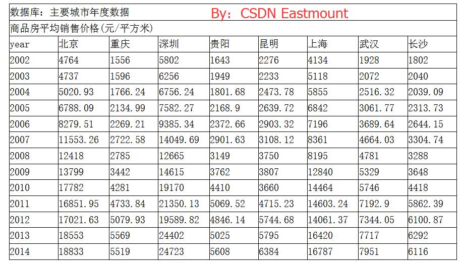
一. Pandas获取数据集并显示
采用Pandas对2002年~2014年的商品房价数据集作时间序列分析,从中抽取几个城市与贵阳做对比,并对贵阳商品房作出分析。
数据集位32.csv,具体值如下:(读者可直接复制)
- year Beijing Chongqing Shenzhen Guiyang Kunming Shanghai Wuhai Changsha
- 2002 4764.00 1556.00 5802.00 1643.00 2276.00 4134.00 1928.00 1802.00
- 2003 4737.00 1596.00 6256.00 1949.00 2233.00 5118.00 2072.00 2040.00
- 2004 5020.93 1766.24 6756.24 1801.68 2473.78 5855.00 2516.32 2039.09
- 2005 6788.09 2134.99 7582.27 2168.90 2639.72 6842.00 3061.77 2313.73
- 2006 8279.51 2269.21 9385.34 2372.66 2903.32 7196.00 3689.64 2644.15
- 2007 11553.26 2722.58 14049.69 2901.63 3108.12 8361.00 4664.03 3304.74
- 2008 12418.00 2785.00 12665.00 3149.00 3750.00 8195.00 4781.00 3288.00
- 2009 13799.00 3442.00 14615.00 3762.00 3807.00 12840.00 5329.00 3648.00
- 2010 17782.00 4281.00 19170.00 4410.00 3660.00 14464.00 5746.00 4418.00
- 2011 16851.95 4733.84 21350.13 5069.52 4715.23 14603.24 7192.90 5862.39
- 2012 17021.63 5079.93 19589.82 4846.14 5744.68 14061.37 7344.05 6100.87
- 2013 18553.00 5569.00 24402.00 5025.00 5795.00 16420.00 7717.00 6292.00
- 2014 18833.00 5519.00 24723.00 5608.00 6384.00 16787.00 7951.00 6116.00
绘制对比各个城市的商品房价数据代码如下所示:
- # -*- coding: utf-8 -*-
- """
- Created on Mon Mar 06 10:55:17 2017
- @author: eastmount
- """
- import pandas as pd
- data = pd.read_csv("32.csv",index_col='year') #index_col用作行索引的列名
- #显示前6行数据
- print(data.shape)
- print(data.head(6))
- import matplotlib.pyplot as plt
- plt.rcParams['font.sans-serif'] = ['simHei'] #用来正常显示中文标签
- plt.rcParams['axes.unicode_minus'] = False #用来正常显示负号
- data.plot()
- plt.savefig(u'时序图.png', dpi=500)
- plt.show()
输出如下所示:
1、plt.rcParams显示中文及负号;
2、plt.savefig保存图片至本地;
3、pandas直接读取数据显示绘制图形,index_col获取索引。
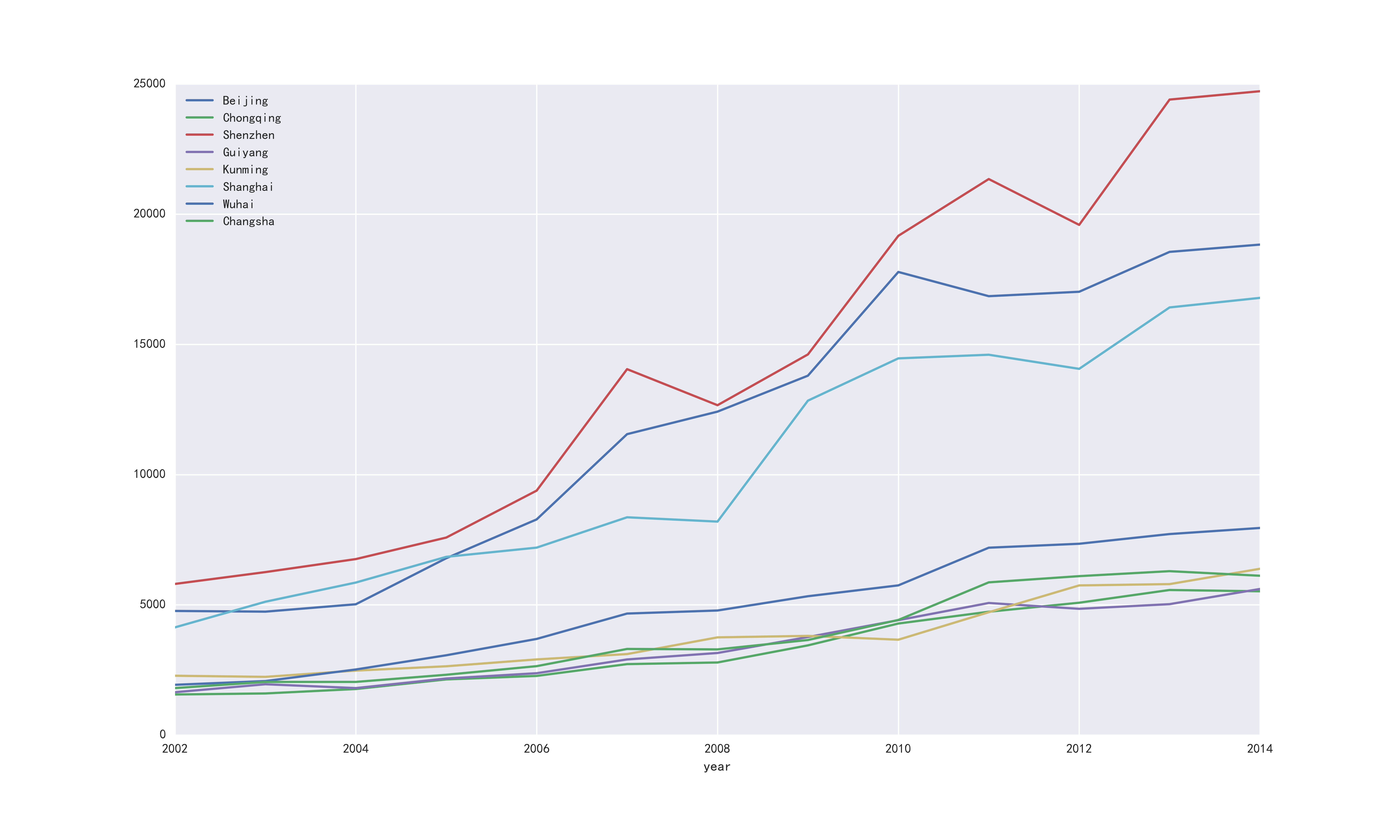
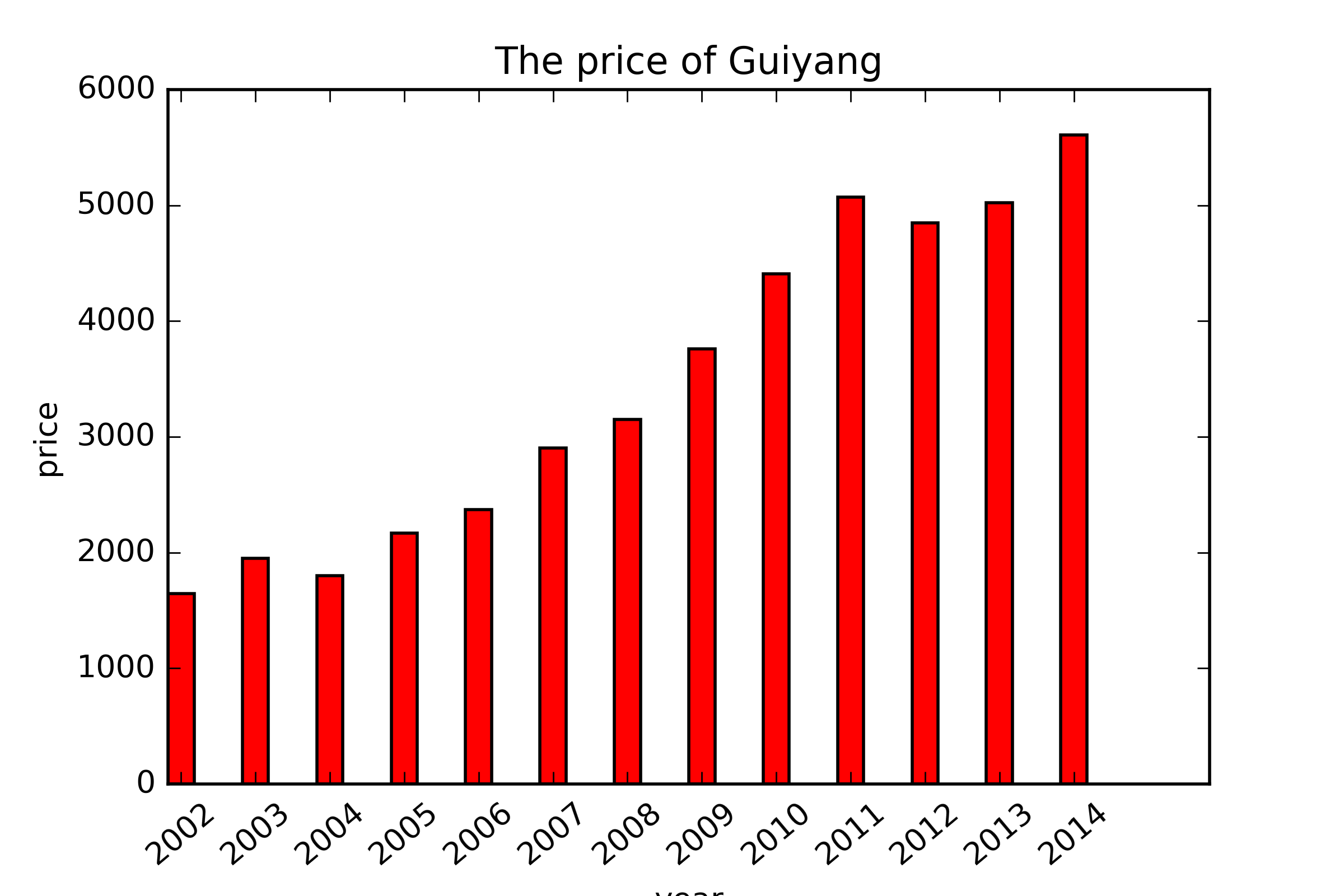
二. Pandas获取某列数据绘制柱状图
接着上面的实验,我们需要获取贵阳那列数据,再绘制相关图形。
- # -*- coding: utf-8 -*-
- """
- Created on Mon Mar 06 10:55:17 2017
- @author: eastmount
- """
- import pandas as pd
- data = pd.read_csv("32.csv",index_col='year') #index_col用作行索引的列名
- #显示前6行数据
- print(data.shape)
- print(data.head(6))
- import matplotlib.pyplot as plt
- plt.rcParams['font.sans-serif'] = ['simHei'] #用来正常显示中文标签
- plt.rcParams['axes.unicode_minus'] = False #用来正常显示负号
- data.plot()
- plt.savefig(u'时序图.png', dpi=500)
- plt.show()
- #获取贵阳数据集并绘图
- gy = data['Guiyang']
- print u'输出贵阳数据'
- print gy
- gy.plot()
- plt.show()
- # -*- coding: utf-8 -*-
- """
- Created on Mon Mar 06 10:55:17 2017
- @author: eastmount
- """
- import pandas as pd
- data = pd.read_csv("32.csv",index_col='year') #index_col用作行索引的列名
- #显示前6行数据
- print(data.shape)
- print(data.head(6))
- #获取贵阳数据集并绘图
- gy = data['Guiyang']
- print u'输出贵阳数据'
- print gy
- import numpy as np
- x = ['2002','2003','2004','2005','2006','2007','2008',
- '2009','2010','2011','2012','2013','2014']
- N = 13
- ind = np.arange(N) #赋值0-13
- width=0.35
- plt.bar(ind, gy, width, color='r', label='sum num')
- #设置底部名称
- plt.xticks(ind+width/2, x, rotation=40) #旋转40度
- plt.title('The price of Guiyang')
- plt.xlabel('year')
- plt.ylabel('price')
- plt.savefig('guiyang.png',dpi=400)
- plt.show()
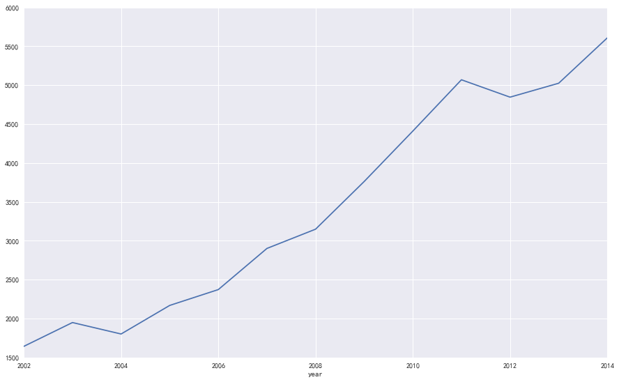
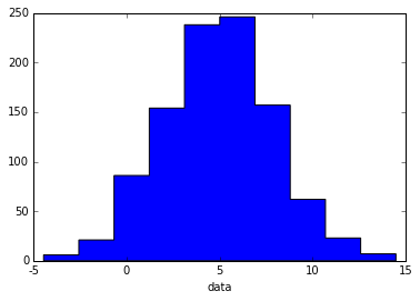
补充一段hist绘制柱状图的代码:
- import numpy as np
- import pylab as pl
- # make an array of random numbers with a gaussian distribution with
- # mean = 5.0
- # rms = 3.0
- # number of points = 1000
- data = np.random.normal(5.0, 3.0, 1000)
- # make a histogram of the data array
- pl.hist(data, histtype='stepfilled') #去掉黑色轮廓
- # make plot labels
- pl.xlabel('data')
- pl.show()
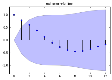
三. Python绘制时间序列-自相关图
核心代码如下所示:
- # -*- coding: utf-8 -*-
- """
- Created on Mon Mar 06 10:55:17 2017
- @author: yxz15
- """
- import pandas as pd
- data = pd.read_csv("32.csv",index_col='year')
- #显示前6行数据
- print(data.shape)
- print(data.head(6))
- import matplotlib.pyplot as plt
- plt.rcParams['font.sans-serif'] = ['simHei']
- plt.rcParams['axes.unicode_minus'] = False
- data.plot()
- plt.savefig(u'时序图.png', dpi=500)
- plt.show()
- from statsmodels.graphics.tsaplots import plot_acf
- gy = data['Guiyang']
- print gy
- plot_acf(gy).show()
- plt.savefig(u'贵阳自相关图',dpi=300)
- from statsmodels.tsa.stattools import adfuller as ADF
- print 'ADF:',ADF(gy)
时间序列相关文章推荐:
python时间序列分析
个股与指数的回归分析(python)
Python_Statsmodels包_时间序列分析_ARIMA模型
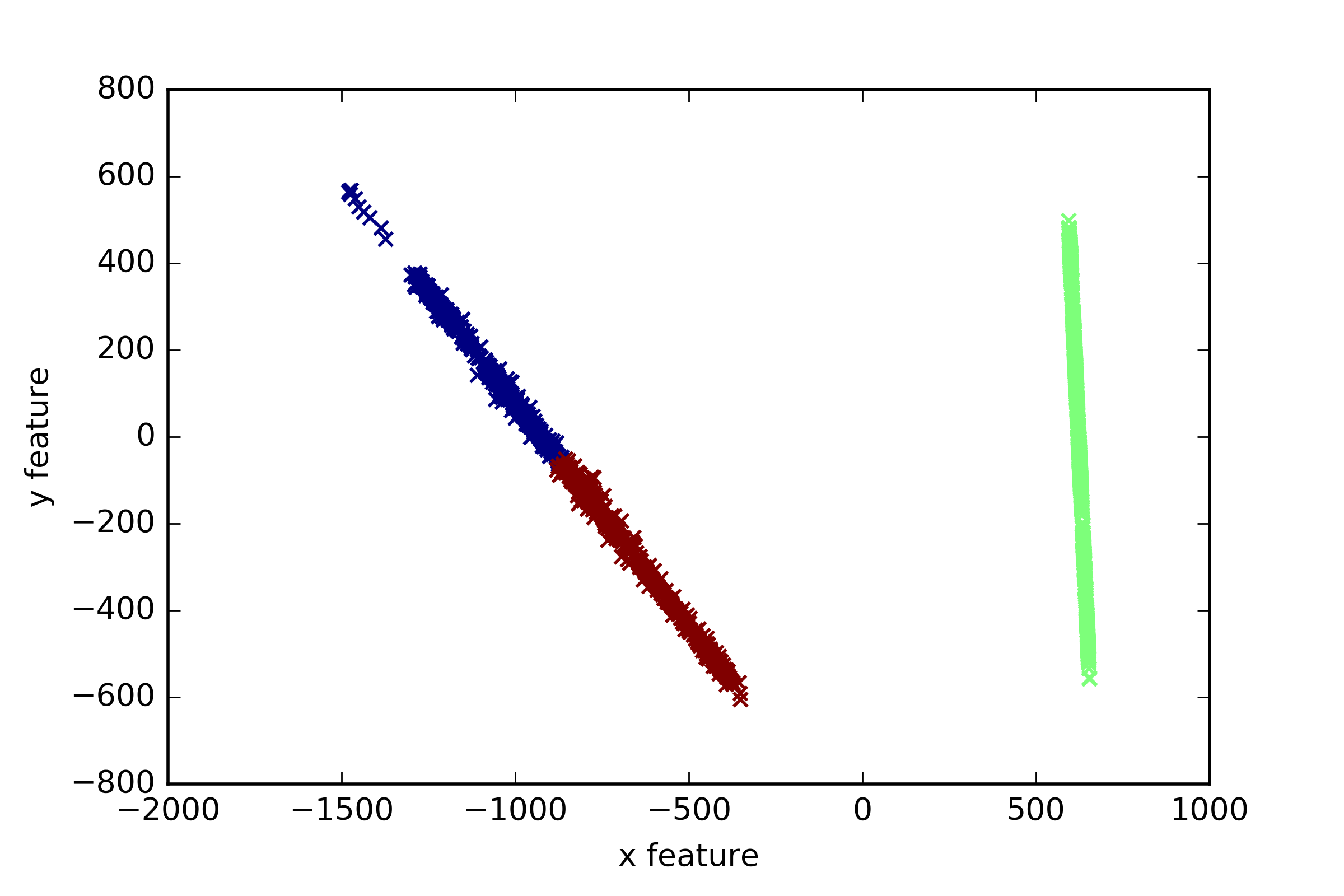
四. 聚类分析大连交易所数据集
这部分主要提供一个网址给大家下载数据集,前面文章说过sklearn自带一些数据集以及UCI官网提供大量的数据集。这里讲述一个大连商品交易所的数据集。
地址:http://www.dce.com.cn/dalianshangpin/xqsj/lssj/index.html#
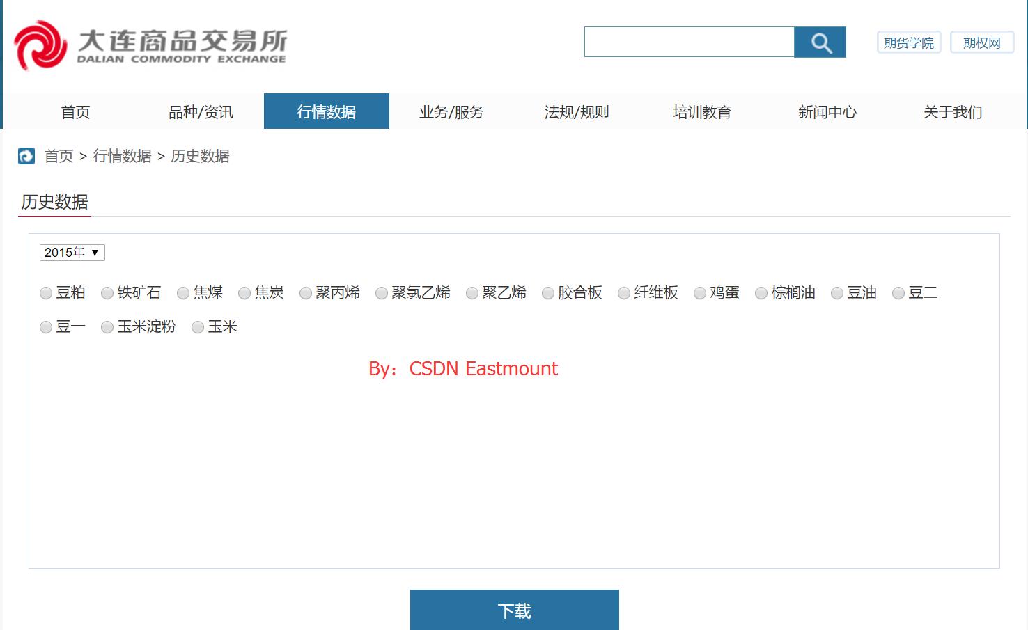
比如下载"焦炭"数据集,命名为"35.csv",在对其进行聚类分析。
- # -*- coding: utf-8 -*-
- """
- Created on Mon Mar 06 10:19:15 2017
- @author: yxz15
- """
- #第一部分:导入数据集
- import pandas as pd
- Coke1 =pd.read_csv("35.csv")
- print Coke1 [:4]
- #第二部分:聚类
- from sklearn.cluster import KMeans
- clf=KMeans(n_clusters=3)
- pre=clf.fit_predict(Coke1)
- print pre[:4]
- #第三部分:降维
- from sklearn.decomposition import PCA
- pca=PCA(n_components=2)
- newData=pca.fit_transform(Coke1)
- print newData[:4]
- x1=[n[0] for n in newData]
- x2=[n[1] for n in newData]
- #第四部分:用matplotlib包画图
- import matplotlib.pyplot as plt
- plt.title
- plt.xlabel("x feature")
- plt.ylabel("y feature")
- plt.scatter(x1,x2,c=pre, marker='x')
- plt.savefig("bankloan.png",dpi=400)
- plt.show()
五. PCA降维及绘图代码
PCA降维绘图参考这篇博客。
http://blog.csdn.net/xiaolewennofollow/article/details/46127485
代码如下:
- # -*- coding: utf-8 -*-
- """
- Created on Mon Mar 06 21:47:46 2017
- @author: yxz
- """
- from numpy import *
- def loadDataSet(fileName,delim='\t'):
- fr=open(fileName)
- stringArr=[line.strip().split(delim) for line in fr.readlines()]
- datArr=[map(float,line) for line in stringArr]
- return mat(datArr)
- def pca(dataMat,topNfeat=9999999):
- meanVals=mean(dataMat,axis=0)
- meanRemoved=dataMat-meanVals
- covMat=cov(meanRemoved,rowvar=0)
- eigVals,eigVets=linalg.eig(mat(covMat))
- eigValInd=argsort(eigVals)
- eigValInd=eigValInd[:-(topNfeat+1):-1]
- redEigVects=eigVets[:,eigValInd]
- print meanRemoved
- print redEigVects
- lowDDatMat=meanRemoved*redEigVects
- reconMat=(lowDDatMat*redEigVects.T)+meanVals
- return lowDDatMat,reconMat
- dataMat=loadDataSet('41.txt')
- lowDMat,reconMat=pca(dataMat,1)
- def plotPCA(dataMat,reconMat):
- import matplotlib
- import matplotlib.pyplot as plt
- datArr=array(dataMat)
- reconArr=array(reconMat)
- n1=shape(datArr)[0]
- n2=shape(reconArr)[0]
- xcord1=[];ycord1=[]
- xcord2=[];ycord2=[]
- for i in range(n1):
- xcord1.append(datArr[i,0]);ycord1.append(datArr[i,1])
- for i in range(n2):
- xcord2.append(reconArr[i,0]);ycord2.append(reconArr[i,1])
- fig=plt.figure()
- ax=fig.add_subplot(111)
- ax.scatter(xcord1,ycord1,s=90,c='red',marker='^')
- ax.scatter(xcord2,ycord2,s=50,c='yellow',marker='o')
- plt.title('PCA')
- plt.savefig('ccc.png',dpi=400)
- plt.show()
- plotPCA(dataMat,reconMat)
数据集为41.txt,值如下:
- 61.5 55
- 59.8 61
- 56.9 65
- 62.4 58
- 63.3 58
- 62.8 57
- 62.3 57
- 61.9 55
- 65.1 61
- 59.4 61
- 64 55
- 62.8 56
- 60.4 61
- 62.2 54
- 60.2 62
- 60.9 58
- 62 54
- 63.4 54
- 63.8 56
- 62.7 59
- 63.3 56
- 63.8 55
- 61 57
- 59.4 62
- 58.1 62
- 60.4 58
- 62.5 57
- 62.2 57
- 60.5 61
- 60.9 57
- 60 57
- 59.8 57
- 60.7 59
- 59.5 58
- 61.9 58
- 58.2 59
- 64.1 59
- 64 54
- 60.8 59
- 61.8 55
- 61.2 56
- 61.1 56
- 65.2 56
- 58.4 63
- 63.1 56
- 62.4 58
- 61.8 55
- 63.8 56
- 63.3 60
- 60.7 60
- 60.9 61
- 61.9 54
- 60.9 55
- 61.6 58
- 59.3 62
- 61 59
- 59.3 61
- 62.6 57
- 63 57
- 63.2 55
- 60.9 57
- 62.6 59
- 62.5 57
- 62.1 56
- 61.5 59
- 61.4 56
- 62 55.3
- 63.3 57
- 61.8 58
- 60.7 58
- 61.5 60
- 63.1 56
- 62.9 59
- 62.5 57
- 63.7 57
- 59.2 60
- 59.9 58
- 62.4 54
- 62.8 60
- 62.6 59
- 63.4 59
- 62.1 60
- 62.9 58
- 61.6 56
- 57.9 60
- 62.3 59
- 61.2 58
- 60.8 59
- 60.7 58
- 62.9 58
- 62.5 57
- 55.1 69
- 61.6 56
- 62.4 57
- 63.8 56
- 57.5 58
- 59.4 62
- 66.3 62
- 61.6 59
- 61.5 58
- 63.2 56
- 59.9 54
- 61.6 55
- 61.7 58
- 62.9 56
- 62.2 55
- 63 59
- 62.3 55
- 58.8 57
- 62 55
- 61.4 57
- 62.2 56
- 63 58
- 62.2 59
- 62.6 56
- 62.7 53
- 61.7 58
- 62.4 54
- 60.7 58
- 59.9 59
- 62.3 56
- 62.3 54
- 61.7 63
- 64.5 57
- 65.3 55
- 61.6 60
- 61.4 56
- 59.6 57
- 64.4 57
- 65.7 60
- 62 56
- 63.6 58
- 61.9 59
- 62.6 60
- 61.3 60
- 60.9 60
- 60.1 62
- 61.8 59
- 61.2 57
- 61.9 56
- 60.9 57
- 59.8 56
- 61.8 55
- 60 57
- 61.6 55
- 62.1 64
- 63.3 59
- 60.2 56
- 61.1 58
- 60.9 57
- 61.7 59
- 61.3 56
- 62.5 60
- 61.4 59
- 62.9 57
- 62.4 57
- 60.7 56
- 60.7 58
- 61.5 58
- 59.9 57
- 59.2 59
- 60.3 56
- 61.7 60
- 61.9 57
- 61.9 55
- 60.4 59
- 61 57
- 61.5 55
- 61.7 56
- 59.2 61
- 61.3 56
- 58 62
- 60.2 61
- 61.7 55
- 62.7 55
- 64.6 54
- 61.3 61
- 63.7 56.4
- 62.7 58
- 62.2 57
- 61.6 56
- 61.5 57
- 61.8 56
- 60.7 56
- 59.7 60.5
- 60.5 56
- 62.7 58
- 62.1 58
- 62.8 57
- 63.8 58
- 57.8 60
- 62.1 55
- 61.1 60
- 60 59
- 61.2 57
- 62.7 59
- 61 57
- 61 58
- 61.4 57
- 61.8 61
- 59.9 63
- 61.3 58
- 60.5 58
- 64.1 59
- 67.9 60
- 62.4 58
- 63.2 60
- 61.3 55
- 60.8 56
- 61.7 56
- 63.6 57
- 61.2 58
- 62.1 54
- 61.5 55
- 61.4 59
- 61.8 60
- 62.2 56
- 61.2 56
- 60.6 63
- 57.5 64
- 61.3 56
- 57.2 62
- 62.9 60
- 63.1 58
- 60.8 57
- 62.7 59
- 62.8 60
- 55.1 67
- 61.4 59
- 62.2 55
- 63 54
- 63.7 56
- 63.6 58
- 62 57
- 61.5 56
- 60.5 60
- 61.1 60
- 61.8 56
- 63.3 56
- 59.4 64
- 62.5 55
- 64.5 58
- 62.7 59
- 64.2 52
- 63.7 54
- 60.4 58
- 61.8 58
- 63.2 56
- 61.6 56
- 61.6 56
- 60.9 57
- 61 61
- 62.1 57
- 60.9 60
- 61.3 60
- 65.8 59
- 61.3 56
- 58.8 59
- 62.3 55
- 60.1 62
- 61.8 59
- 63.6 55.8
- 62.2 56
- 59.2 59
- 61.8 59
- 61.3 55
- 62.1 60
- 60.7 60
- 59.6 57
- 62.2 56
- 60.6 57
- 62.9 57
- 64.1 55
- 61.3 56
- 62.7 55
- 63.2 56
- 60.7 56
- 61.9 60
- 62.6 55
- 60.7 60
- 62 60
- 63 57
- 58 59
- 62.9 57
- 58.2 60
- 63.2 58
- 61.3 59
- 60.3 60
- 62.7 60
- 61.3 58
- 61.6 60
- 61.9 55
- 61.7 56
- 61.9 58
- 61.8 58
- 61.6 56
- 58.8 66
- 61 57
- 67.4 60
- 63.4 60
- 61.5 59
- 58 62
- 62.4 54
- 61.9 57
- 61.6 56
- 62.2 59
- 62.2 58
- 61.3 56
- 62.3 57
- 61.8 57
- 62.5 59
- 62.9 60
- 61.8 59
- 62.3 56
- 59 70
- 60.7 55
- 62.5 55
- 62.7 58
- 60.4 57
- 62.1 58
- 57.8 60
- 63.8 58
- 62.8 57
- 62.2 58
- 62.3 58
- 59.9 58
- 61.9 54
- 63 55
- 62.4 58
- 62.9 58
- 63.5 56
- 61.3 56
- 60.6 54
- 65.1 58
- 62.6 58
- 58 62
- 62.4 61
- 61.3 57
- 59.9 60
- 60.8 58
- 63.5 55
- 62.2 57
- 63.8 58
- 64 57
- 62.5 56
- 62.3 58
- 61.7 57
- 62.2 58
- 61.5 56
- 61 59
- 62.2 56
- 61.5 54
- 67.3 59
- 61.7 58
- 61.9 56
- 61.8 58
- 58.7 66
- 62.5 57
- 62.8 56
- 61.1 68
- 64 57
- 62.5 60
- 60.6 58
- 61.6 55
- 62.2 58
- 60 57
- 61.9 57
- 62.8 57
- 62 57
- 66.4 59
- 63.4 56
- 60.9 56
- 63.1 57
- 63.1 59
- 59.2 57
- 60.7 54
- 64.6 56
- 61.8 56
- 59.9 60
- 61.7 55
- 62.8 61
- 62.7 57
- 63.4 58
- 63.5 54
- 65.7 59
- 68.1 56
- 63 60
- 59.5 58
- 63.5 59
- 61.7 58
- 62.7 58
- 62.8 58
- 62.4 57
- 61 59
- 63.1 56
- 60.7 57
- 60.9 59
- 60.1 55
- 62.9 58
- 63.3 56
- 63.8 55
- 62.9 57
- 63.4 60
- 63.9 55
- 61.4 56
- 61.9 55
- 62.4 55
- 61.8 58
- 61.5 56
- 60.4 57
- 61.8 55
- 62 56
- 62.3 56
- 61.6 56
- 60.6 56
- 58.4 62
- 61.4 58
- 61.9 56
- 62 56
- 61.5 57
- 62.3 58
- 60.9 61
- 62.4 57
- 55 61
- 58.6 60
- 62 57
- 59.8 58
- 63.4 55
- 64.3 58
- 62.2 59
- 61.7 57
- 61.1 59
- 61.5 56
- 58.5 62
- 61.7 58
- 60.4 56
- 61.4 56
- 61.5 55
- 61.4 56
- 65 56
- 56 60
- 60.2 59
- 58.3 58
- 53.1 63
- 60.3 58
- 61.4 56
- 60.1 57
- 63.4 55
- 61.5 59
- 62.7 56
- 62.5 55
- 61.3 56
- 60.2 56
- 62.7 57
- 62.3 58
- 61.5 56
- 59.2 59
- 61.8 59
- 61.3 55
- 61.4 58
- 62.8 55
- 62.8 64
- 62.4 61
- 59.3 60
- 63 60
- 61.3 60
- 59.3 62
- 61 57
- 62.9 57
- 59.6 57
- 61.8 60
- 62.7 57
- 65.3 62
- 63.8 58
- 62.3 56
- 59.7 63
- 64.3 60
- 62.9 58
- 62 57
- 61.6 59
- 61.9 55
- 61.3 58
- 63.6 57
- 59.6 61
- 62.2 59
- 61.7 55
- 63.2 58
- 60.8 60
- 60.3 59
- 60.9 60
- 62.4 59
- 60.2 60
- 62 55
- 60.8 57
- 62.1 55
- 62.7 60
- 61.3 58
- 60.2 60
- 60.7 56
最后希望这篇文章对你有所帮助,尤其是我的学生和接触数据挖掘、机器学习的博友。这篇文字主要是记录一些代码片段,作为在线笔记,也希望对你有所帮助。
一醉一轻舞,一梦一轮回。一曲一人生,一世一心愿。
(By:Eastmount 2017-03-07 下午3点半 http://blog.csdn.net/eastmount/ )


 795
795

 被折叠的 条评论
为什么被折叠?
被折叠的 条评论
为什么被折叠?
 到【灌水乐园】发言


