


只是不知道单片机是否跑得动……
以下内容摘自维基百科
卡尔曼滤波是一种高效率的递归滤波器(自回归滤波器), 它能够从一系列的不完全包含噪声的测量(英文:measurement)中,估计动态系统的状态。
目录[隐藏] |
[编辑] 应用实例
卡尔曼滤波的一个典型实例是从一组有限的,包含噪声的,对物体位置的观察序列(可能有偏差)预测出物体的位置的坐标及速度. 在很多工程应用(如雷达, 计算机视觉)中都可以找到它的身影. 同时,卡尔曼滤波也是控制理论以及控制系统工程中的一个重要课题.
例如,对于雷达来说,人们感兴趣的是其能够跟踪目标.但目标的位置,速度,加速度的测量值往往在任何时候都有噪声.卡尔曼滤波利用目标的动态信息,设法去掉噪声的影响,得到一个关于目标位置的好的估计。这个估计可以是对当前目标位置的估计(滤波),也可以是对于将来位置的估计(预测),也可以是对过去位置的估计(插值或平滑).
[编辑] 命名
这种滤波方法以它的发明者鲁道夫.E.卡尔曼(Rudolph E. Kalman)命名,但是根据文献可知实际上Peter Swerling在更早之前就提出了一种类似的算法。
斯坦利.施密特(Stanley Schmidt)首次实现了卡尔曼滤波器。卡尔曼在NASA埃姆斯研究中心访问时,发现他的方法对于解决阿波罗计划的轨道预测很有用,后来阿波罗飞船的导航电脑便使用了这种滤波器。 关于这种滤波器的论文由Swerling (1958)、Kalman (1960)与 Kalman and Bucy (1961)发表。
目前,卡尔曼滤波已经有很多不同的实现.卡尔曼最初提出的形式现在一般称为简单卡尔曼滤波器。除此以外,还有施密特扩展滤波器,信息滤波器以及很多Bierman, Thornton 开发的平方根滤波器的变种。也许最常见的卡尔曼滤波器是锁相环,它在收音机、计算机和几乎任何视频或通讯设备中广泛存在。
以下的讨论需要线性代数以及概率论的一般知识。
[编辑] 基本动态系统模型
卡尔曼滤波建立在线性代数和隐马尔可夫模型(hidden Markov model)上。其基本动态系统可以用一个马尔可夫链表示,该马尔可夫链建立在一个被高斯噪声(即正态分布的噪声)干扰的线性算子上的。系统的状态可以用一个元素为实数的向量表示。 随着离散时间的每一个增加,这个线性算子就会作用在当前状态上,产生一个新的状态,并也会带入一些噪声,同时系统的一些已知的控制器的控制信息也会被加入。同时,另一个受噪声干扰的线性算子产生出这些隐含状态的可见输出。
为了从一系列有噪声的观察数据中用卡尔曼滤波器估计出被观察过程的内部状态,我们必须把这个过程在卡尔曼滤波的框架下建立模型。也就是说对于每一步k,定义矩阵Fk, Hk, Qk, Rk,有时也需要定义Bk,如下。

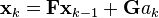
卡尔曼滤波模型假设k时刻的真实状态是从(k − 1)时刻的状态演化而来,符合下式
:
其中

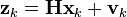
时刻k,对真实状态 xk的一个测量zk满足下式:
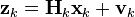
其中Hk是观测模型,它把真实状态空间映射成观测空间,vk 是观测噪声,其均值为零,协方差为Rk,且服从正态分布。

初始状态以及每一时刻的噪声{x0, w1, ..., wk, v1 ... vk} 都为认为是互相独立的.
实际上,很多真实世界的动态系统都并不确切的符合这个模型;但是由于卡尔曼滤波器被设计在有噪声的情况下工作,一个近似的符合已经可以使这个滤波器非常有用了。更多其它更复杂的卡尔曼滤波器的变种,在下边讨论中有描述。
[编辑] 卡尔曼滤波器
卡尔曼滤波是一种递归的估计,即只要获知上一时刻状态的估计值以及当前状态的观测值就可以计算出当前状态的估计值,因此不需要记录观测或者估计的历史信息。卡尔曼滤波器与大多数滤波器不同之处,在于它是一种纯粹的时域滤波器,它不需要像低通滤波器等频域滤波器那样,需要在频域设计再转换到时域实现。
卡尔曼滤波器的状态由以下两个变量表示:
 ,在时刻k 的状态的估计;
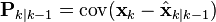
  ,误差相关矩阵,度量估计值的精确程度。
卡尔曼滤波器的操作包括两个阶段:预测与更新。在预测阶段,滤波器使用上一状态的估计,做出对当前状态的估计。在更新阶段,滤波器利用对当前状态的观测值优化在预测阶段获得的预测值,以获得一个更精确的新估计值。
[编辑] 预测
-
 (预测状态)
-
 (预测估计协方差)
[编辑] 更新
-
 (测量革新或余量,英文分别为measurement innovation与residual,请见
[1])
(测量革新或余量,英文分别为measurement innovation与residual,请见
[1])
-
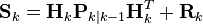 (测量革新(余量)协方差)
-
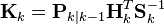 (卡尔曼增益)
-
 (更新的状态估计)
-
 (更新的协方差估计)
使用上述公式计算仅在最优卡尔曼增益的时候有效。使用其他增益的话,公式要复杂一些,请参见推导。
[编辑] 不变量(Invariant)
如果模型准确,那么 与
与 的值准确的反映了最初状态的分布,那么以下的不变量就得到了保存:所有估计的均值都为零
![/textrm{E}[/textbf{x}_k - /hat{/textbf{x}}_{k|k}] = /textrm{E}[/textbf{x}_k - /hat{/textbf{x}}_{k|k-1}] = 0](http://upload.wikimedia.org/math/4/c/4/4c4bbb2da083dae032f5a7930e7b5d80.png)
![/textrm{E}[/tilde{/textbf{y}}_k] = 0](http://upload.wikimedia.org/math/0/0/7/00703cccab98e464367ae2b34e9b1493.png)
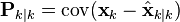
并且 协方差矩阵 准确的反映了以下估计的协方差:

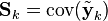
请注意,其中![/textrm{E}[/textbf{a}] = 0](http://upload.wikimedia.org/math/b/6/f/b6f3a97034c8cef749d075ec49478bc0.png) ,
, ![/textrm{cov}(/textbf{a}) = /textrm{E}[/textbf{a}/textbf{a}^T]](http://upload.wikimedia.org/math/d/2/7/d27f414efcd30770cfb2e541b1a61972.png) 。
。
[编辑] 实例
考虑在无摩擦的、无限长的直轨道上的一辆车。该车最初停在位置 0 处,但时不时受到随机的冲击。我们每隔Δt秒即测量车的位置,但是这个测量是非精确的;我们想建立一个关于其位置以及速度的模型。我们来看如何推导出这个模型以及如何从这个模型得到卡尔曼滤波器。
因为车上无动力,所以我们可以忽略掉Bk 和uk。由于F、H、R 和Q 是常数,所以时间下标可以去掉。
车的位置以及速度(或者更加一般的,一个粒子的运动状态)可以被线性状态空间描述如下:

其中 是速度,也就是位置对于时间的导数。
我们假设在(k − 1)时刻与k时刻之间,车受到ak的加速度,其符合均值为0,标准差为σa的正态分布。根据牛顿运动定律,我们可以推出
其中

且

我们可以发现
-
![/textbf{Q} = /textrm{cov}(/textbf{G}a) = /textrm{E}[(/textbf{G}a)(/textbf{G}a)^{T}] = /textbf{G} /textrm{E}[a^2] /textbf{G}^{T} = /textbf{G}[/sigma_a^2]/textbf{G}^{T} = /sigma_a^2 /textbf{G}/textbf{G}^{T}](http://upload.wikimedia.org/math/d/e/e/dee0b505f8b7b5270725e5f544fb53e4.png) (因为
σ
a 是一个标量).
(因为
σ
a 是一个标量).
在每一时刻,我们对其位置进行测量,测量受到噪声干扰.我们假设噪声服从正态分布,均值为0,标准差为σz。
其中

且
![/textbf{R} = /textrm{E}[/textbf{v}_k /textbf{v}_k^{T}] = /begin{bmatrix} /sigma_z^2 /end{bmatrix}](http://upload.wikimedia.org/math/b/c/3/bc31fd596ea83fc789506857ab672644.png)
如果我们知道足够精确的车最初的位置,那么我们可以初始化

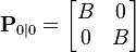
并且,我们告诉滤波器我们知道确切的初始位置,我们给出一个协方差矩阵:
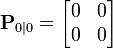
如果我们不确切的知道最初的位置与速度,那么协方差矩阵可以初始化为一个对角线元素是B的矩阵,B取一个合适的比较大的数。
此时,与使用模型中已有信息相比,滤波器更倾向于使用初次测量值的信息。
[编辑] 推导
[编辑] 推导后验协方差矩阵
按照上边的定义,我们从误差协方差Pk|k开始推导如下:
代入

再代入 

与 

整理误差向量,得

因为测量误差vk 与其他项是非相关的,因此有

利用协方差矩阵的性质,此式可以写作

使用不变量Pk|k-1以及Rk的定义 这一项可以写作 : 这一公式对于任何卡尔曼增益Kk都成立。如果Kk是最优卡尔曼增益,则可以进一步简化,请见下文。
[编辑] 最优卡尔曼增益的推导
卡尔曼滤波器是一个最小均方误差估计器,后验状态误差估计(英文:posteriori state estimate)是

我们最小化这个矢量幅度平方的期望值,![/textrm{E}[|/textbf{x}_{k} - /hat{/textbf{x}}_{k|k}|^2]](http://upload.wikimedia.org/math/d/a/c/dac65520055c06e789c58462cc7b7738.png) ,这等同于最小化后验估计协方差矩阵 Pk|k的迹(trace)。将上面方程中的项展开、抵消,得到:
,这等同于最小化后验估计协方差矩阵 Pk|k的迹(trace)。将上面方程中的项展开、抵消,得到:


当矩阵导数是 0 的时候得到迹(trace)的最小值:

从这个方程解出卡尔曼增益Kk:


这个增益称为最优卡尔曼增益,在使用时得到最小均方误差。
[编辑] 后验误差协方差公式的化简
在卡尔曼增益等于上面导出的最优值时,计算后验协方差的公式可以进行简化。在卡尔曼增益公式两侧的右边都乘以 SkKkT 得到
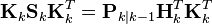
根据上面后验误差协方差展开公式,

最后两项可以抵消,得到
-
 .
.
这个公式的计算比较简单,所以实际中总是使用这个公式,但是需注意这公式仅在使用最优卡尔曼增益的时候它才成立。如果算术精度总是很低而导致numerical stability出现问题,或者特意使用非最优卡尔曼增益,那么就不能使用这个简化;必须使用上面导出的后验误差协方差公式。
[编辑] 与递归Bayesian估计之间的关系
假设真正的状态是无法观察的马尔科夫过程,测量结果是从隐性马尔科夫模型观察到的状态。
根据马尔科夫假设,真正的状态仅受最近一个状态影响而与其它以前状态无关。

与此类似,在时刻 k 测量只与当前状态有关而与其它状态无关。

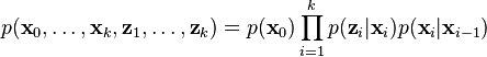
根据这些假设,隐性马尔科夫模型所有状态的概率分布可以简化为:
However, when the Kalman filter is used to estimate the state x, the probability distribution of interest is that associated with the current states conditioned on the measurements up to the current timestep. (This is achieved by marginalizing out the previous states and dividing by the probability of the measurement set.) 但是,当卡尔曼滤波器用来估计状态x的时候,
This leads to the predict and update steps of the Kalman filter written probabilistically. The probability distribution associated with the predicted state is product of the probability distribution associated with the transition from the (k − 1)th timestep to the kth and the probability distribution associated with the previous state, with the true state at (k − 1) integrated out.

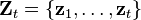
The measurement set up to time t is
The probability distribution of updated is proportional to the product of the measurement likelihood and the predicted state.

The denominator

is an unimportant normalization term.
The remaining probability density functions are


Note that the PDF at the previous timestep is inductively assumed to be the estimated state and covariance. This is justified because, as an optimal estimator, the Kalman filter makes best use of the measurements, therefore the PDF for  given the measurements
  is the Kalman filter estimate.
[编辑] 信息滤波器
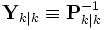
In the information filter, or inverse covariance filter, the estimated covariance and estimated state are replaced by the information matrix and information vector respectively.

Similarly the predicted covariance and state have equivalent information forms,


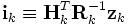
as have the measurement covariance and measurement vector.

The information update now becomes a trivial sum.


The main advantage of the information filter is that N measurements can be filtered at each timestep simply by summing their information matrices and vectors.


To predict the information filter the information matrix and vector can be converted back to their state space equivalents, or alternatively the information space prediction can be used.
![/textbf{M}_{k} = [/textbf{F}_{k}^{-1}]^{T} /textbf{Y}_{k|k} /textbf{F}_{k}^{-1}](http://upload.wikimedia.org/math/4/6/2/462faaf7535ba2354a977b44b13a45b6.png)
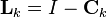
![/textbf{C}_{k} = /textbf{M}_{k} [/textbf{M}_{k}+/textbf{Q}_{k}^{-1}]^{-1}](http://upload.wikimedia.org/math/b/a/b/baba972b698cfcfce00c6fdb6c3c52e9.png)

![/hat{/textbf{y}}_{k|k-1} = /textbf{L}_{k} [/textbf{F}_{k}^{-1}]^{T}/hat{/textbf{y}}_{k|k}](http://upload.wikimedia.org/math/0/9/9/0995a9549f9eda92c179c5833690b88b.png)
Note that if F and Q are time invariant these values can be cached. Note also that F and Q need to be invertible.
[编辑] 非线性滤波器
基本卡尔曼滤波器(The basic Kalman filter)是限制在线性的假设之下。然而,大部份非平凡的(non-trial)的系统都是非线性系统。其中的“非线性性质”(non- linearity )可能是伴随存在过程模型(process model)中或观测模型(observation model)中,或者两者兼有之。
[编辑] 扩展卡尔曼滤波器
在扩展卡尔曼滤波器(EKF)中状态转换和观测模型不需要是状态的线性函数,可替换为(可微的)函数。


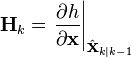
函数 f 可以用来从过去的估计值中计算预测的状态,相似的,函数 h可以用来以预测的状态计算预测的测量值。然而 f 和 h 不能直接的应用在协方差中,取而代之的是计算偏导矩阵(Jacobian)。
在每一步中使用当前的估计状态计算Jacobian矩阵,这几个矩阵可以用在卡尔曼滤波器的方程中。这个过程,实质上将非线性的函数在当前估计值处线性化了。
这样一来,卡尔曼滤波器的等式为:
预测

使用Jacobians矩阵更新模型

更新

[编辑] Unscented Kalman filter
The extended Kalman filter gives particularly poor performance on highly non-linear functions because only the mean is propagated through the non-linearity. The unscented Kalman filter (UKF) [JU97] uses a deterministic sampling technique to pick a minimal set of sample points (called sigma points) around the mean. These sigma points are then propagated through the non-linear functions and the covariance of the estimate is then recovered. The result is a filter which more accurately captures the true mean and covariance. (This can be verified using Monte Carlo sampling or through a Taylor series expansion of the posterior statistics.) In addition, this technique removes the requirement to analytically calculate Jacobians, which for complex functions can be a difficult task in itself.
预测
如同扩展卡尔曼滤波器(EKF)一样, UKF的预测过程可以独立于UKF的更新过程之外,与一个线性的(或者确实是扩展卡尔曼滤波器的)更新过程合并来使用;或者,UKF的预测过程与更新过程在上述中地位互换亦可。
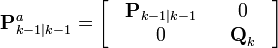
The estimated state and covariance are augmented with the mean and covariance of the process noise.
![/textbf{x}_{k-1|k-1}^{a} = [ /hat{/textbf{x}}_{k-1|k-1}^{T} /quad E[/textbf{w}_{k}^{T}] / ]^{T}](http://upload.wikimedia.org/math/7/c/0/7c0c53eef72ef92fff5265ffd5a5f68d.png)
A set of 2L+1 sigma points is derived from the augmented state and covariance where L is the dimension of the augmented state.


The sigma points are propagated through the transition function f.

The weighted sigma points are recombined to produce the predicted state and covariance.
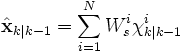
![/textbf{P}_{k|k-1} = /sum_{i=1}^N W_{c}^{i}/ [/chi_{k|k-1}^{i} - /hat{/textbf{x}}_{k|k-1}] [/chi_{k|k-1}^{i} - /hat{/textbf{x}}_{k|k-1}]^{T}](http://upload.wikimedia.org/math/4/e/a/4ea9c706f681af110c4bca7161594675.png)
Where the weights for the state and covariance are given are:


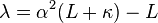
Typical values for α, β, and κ are 10 − 3, 2 and 0 respectively. (These values should suffice for most purposes.)
更新
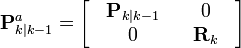
The predicted state and covariance are augmented as before, except now with the mean and covariance of the measurement noise.
![/textbf{x}_{k|k-1}^{a} = [ /hat{/textbf{x}}_{k|k-1}^{T} /quad E[/textbf{v}_{k}^{T}] / ]^{T}](http://upload.wikimedia.org/math/f/a/6/fa6d80e1bb88f3fe9739339130520c8d.png)
As before, a set of 2L + 1 sigma points is derived from the augmented state and covariance where L is the dimension of the augmented state.


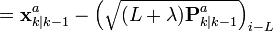
Alternatively if the UKF prediction has been used the sigma points themselves can be augmented along the following lines
![/chi_{k|k-1} := [ /chi_{k|k-1} /quad E[/textbf{v}_{k}^{T}] / ]^{T} /pm /sqrt{ (L + /lambda) /textbf{R}_{k}^{a} }](http://upload.wikimedia.org/math/4/4/b/44b1cd58525d54f78a6ae03e529b9684.png)
where

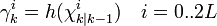
The sigma points are projected through the observation function h.
The weighted sigma points are recombined to produce the predicted measurement and predicted measurement covariance.

![/textbf{P}_{z_{k}z_{k}} = /sum_{i=1}^N W_{c}^{i}/ [/gamma_{k}^{i} - /hat{/textbf{z}}_{k}] [/gamma_{k}^{i} - /hat{/textbf{z}}_{k}]^{T}](http://upload.wikimedia.org/math/5/e/9/5e9ac4981382edde1002d80c968e14c4.png)
The state-measurement cross-correlation matrix,
![/textbf{P}_{x_{k}z_{k}} = /sum_{i=1}^N W_{c}^{i}/ [/chi_{k|k-1}^{i} - /hat{/textbf{x}}_{k|k-1}] [/gamma_{k}^{i} - /hat{/textbf{z}}_{k}]^{T}](http://upload.wikimedia.org/math/5/d/b/5db22c87d6944777d1e8bcf9657a881b.png)
is used to compute the UKF Kalman gain.

As with the Kalman filter, the updated state is the predicted state plus the innovation weighted by the Kalman gain,

And the updated covariance is the predicted covariance, minus the predicted measurement covariance, weighted by the Kalman gain.

[编辑] 应用
[编辑] 参见
- 快速卡尔曼滤波
- 比较: 维纳滤波及 the multimodal Particle filter estimator.
[编辑] 外部连接
- An Introduction to the Kalman Filter, SIGGRAPH 2001 Course, Greg Welch and Gary Bishop
- Kalman filtering chapter from Stochastic Models, Estimation, by Peter Maybeck
- Kalman Filter webpage, with lots of links
- Kalman Filtering
- The unscented Kalman filter for nonlinear estimation
- Kalman Filters, thorough introduction to several types, together with applications to Robot Localization
[编辑] 参考文献
- Gelb A., editor. Applied optimal estimation. MIT Press, 1974.
- Kalman, R. E. A New Approach to Linear Filtering and Prediction Problems, Transactions of the ASME - Journal of Basic Engineering Vol. 82: pp. 35-45 (1960)
- Kalman, R. E., Bucy R. S., New Results in Linear Filtering and Prediction Theory, Transactions of the ASME - Journal of Basic Engineering Vol. 83: pp. 95-107 (1961)
- [JU97] Julier, Simon J. and Jeffery K. Uhlmann. A New Extension of the Kalman Filter to nonlinear Systems. In The Proceedings of AeroSense: The 11th International Symposium on Aerospace/Defense Sensing,Simulation and Controls, Multi Sensor Fusion, Tracking and Resource Management II, SPIE, 1997.
- Harvey, A.C. Forecasting, Structural Time Series Models and the Kalman Filter. Cambridge University Press, Cambridge, 1989


 2404
2404

 被折叠的 条评论
为什么被折叠?
被折叠的 条评论
为什么被折叠?
 到【灌水乐园】发言


