Andrew Ng Deep Learning 第三周 编程练习 Planar_data_classification_with_one_hidden_layer

Exercise 1

How many training examples do you have? In addition, what is the shape of the variables X and Y?

Hint: How do you get the shape of a numpy array? (help)

# (≈ 3 lines of code)
# shape_X = ...
# shape_Y = ...
# training set size
# m = ...
# YOUR CODE STARTS HERE
shape_X=X.shape
shape_Y=Y.shape
m=shape_X[1]

# YOUR CODE ENDS HERE

print ('The shape of X is: ' + str(shape_X))
print ('The shape of Y is: ' + str(shape_Y))
print ('I have m = %d training examples!' % (m))

Exercise 2 layer_sizes

Define three variables:

• n_x: the size of the input layer
• n_h: the size of the hidden layer (set this to 4)
• n_y: the size of the output layer

Hint: Use shapes of X and Y to find n_x and n_y. Also, hard code the hidden layer size to be 4.

# GRADED FUNCTION: layer_sizes

def layer_sizes(X, Y):
    """
    Arguments:
    X -- input dataset of shape (input size, number of examples)
    Y -- labels of shape (output size, number of examples)
    
    Returns:
    n_x -- the size of the input layer
    n_h -- the size of the hidden layer
    n_y -- the size of the output layer
    """
    #(≈ 3 lines of code)
    # n_x = ... 
    # n_h = ...
    # n_y = ... 
    # YOUR CODE STARTS HERE
    n_x = X.shape[0]
    n_h = 4
    n_y = Y.shape[0]
    
    # YOUR CODE ENDS HERE
    return (n_x, n_h, n_y)

Exercise 3 initialize_parameters

Implement the function initialize_parameters().

Instructions:

• Make sure your parameters’ sizes are right. Refer to the neural network figure above if needed.
• You will initialize the weights matrices with random values.
  • Use: np.random.randn(a,b) * 0.01 to randomly initialize a matrix of shape (a,b).
• You will initialize the bias vectors as zeros.
  • Use: np.zeros((a,b)) to initialize a matrix of shape (a,b) with zeros.

# GRADED FUNCTION: initialize_parameters

def initialize_parameters(n_x, n_h, n_y):
    """
    Argument:
    n_x -- size of the input layer
    n_h -- size of the hidden layer
    n_y -- size of the output layer
    
    Returns:
    params -- python dictionary containing your parameters:
                    W1 -- weight matrix of shape (n_h, n_x)
                    b1 -- bias vector of shape (n_h, 1)
                    W2 -- weight matrix of shape (n_y, n_h)
                    b2 -- bias vector of shape (n_y, 1)
    """    
    #(≈ 4 lines of code)
    # W1 = ...
    # b1 = ...
    # W2 = ...
    # b2 = ...
    # YOUR CODE STARTS HERE
    W1 = np.random.randn(n_h,n_x)* 0.01
    b1 = np.zeros((n_h, 1))
    W2 = np.random.randn(n_y,n_h)* 0.01
    b2 = np.zeros((n_y, 1))
    
    
    # YOUR CODE ENDS HERE

    parameters = {"W1": W1,
                  "b1": b1,
                  "W2": W2,
                  "b2": b2}
    
    return parameters

Exercise 4 forward_propagation

Implement forward_propagation() using the following equations:
$z^{[1]}=w^{[1]}x+b^{[1]}$
$A^{[1]}=tanh(z^{[1]})$
$z^{[2]}=w^{[2]}{A}^{[1]}+b^{[2]}$
$Y=A^{[2]}=\sigma (z^{[2]})$

Instructions:

• Check the mathematical representation of your classifier in the figure above.
• Use the function sigmoid(). It’s built into (imported) this notebook.
• Use the function np.tanh(). It’s part of the numpy library.
• Implement using these steps:
  1.Retrieve each parameter from the dictionary “parameters” (which is the output of initialize_parameters() by using parameters["…"].
  2.Implement Forward Propagation. Compute 𝑍[1],𝐴[1],𝑍[2] and 𝐴[2] (the vector of all your predictions on all the examples in the training set).
• Values needed in the backpropagation are stored in “cache”. The cache will be given as an input to the backpropagation function.

# GRADED FUNCTION:forward_propagation

def forward_propagation(X, parameters):
    """
    Argument:
    X -- input data of size (n_x, m)
    parameters -- python dictionary containing your parameters (output of initialization function)
    
    Returns:
    A2 -- The sigmoid output of the second activation
    cache -- a dictionary containing "Z1", "A1", "Z2" and "A2"
    """
    # Retrieve each parameter from the dictionary "parameters"
    #(≈ 4 lines of code)
    # W1 = ...
    # b1 = ...
    # W2 = ...
    # b2 = ...
    # YOUR CODE STARTS HERE
    W1 = parameters["W1"]
    b1 = parameters["b1"]
    W2 = parameters["W2"]
    b2 = parameters["b2"]
    # YOUR CODE ENDS HERE
    
    # Implement Forward Propagation to calculate A2 (probabilities)
    # (≈ 4 lines of code)
    # Z1 = ...
    # A1 = ...
    # Z2 = ...
    # A2 = ...
    # YOUR CODE STARTS HERE
    Z1 = np.dot(W1, X)+b1
    A1 = np.tanh(Z1)
    Z2 = np.dot(W2, A1)+b2
    A2 = sigmoid(Z2)
    
    # YOUR CODE ENDS HERE
    
    assert(A2.shape == (1, X.shape[1]))
    
    cache = {"Z1": Z1,
             "A1": A1,
             "Z2": Z2,
             "A2": A2}
    
    return A2, cache

Exercise 5 compute_cost

Implement compute_cost() to compute the value of the cost $J$ .

Instructions:

• There are many ways to implement the cross-entropy loss. This is one way to implement one part of the equation without for loops: $-{\sum }_{i=1}^m{y}^{(i)}log(a^{[2](i)}):$

logprobs = np.multiply(np.log(A2),Y)

cost = - np.sum(logprobs)

• Use that to build the whole expression of the cost function.

Notes:

• You can use either np.multiply() and then np.sum() or directly np.dot()).
• If you use np.multiply followed by np.sum the end result will be a type float, whereas if you use np.dot, the result will be a 2D numpy array.
• You can use np.squeeze() to remove redundant dimensions (in the case of single float, this will be reduced to a zero-dimension array).
• You can also cast the array as a type float using float().

# GRADED FUNCTION: compute_cost

def compute_cost(A2, Y):
    """
    Computes the cross-entropy cost given in equation (13)
    
    Arguments:
    A2 -- The sigmoid output of the second activation, of shape (1, number of examples)
    Y -- "true" labels vector of shape (1, number of examples)

    Returns:
    cost -- cross-entropy cost given equation (13)
    
    """
    
    m = Y.shape[1] # number of examples

    # Compute the cross-entropy cost
    # (≈ 2 lines of code)
    # logprobs = ...
    # cost = ...
    # YOUR CODE STARTS HERE
    logprobs = np.dot(Y,np.log(A2).T) + np.dot((1-Y),np.log(1-A2).T)
    cost = -1/m * np.sum(logprobs)
    
    # YOUR CODE ENDS HERE
    
    cost = float(np.squeeze(cost))  # makes sure cost is the dimension we expect. 
                                    # E.g., turns [[17]] into 17 
    
    return cost

Exercise 6 backward_propagation

Implement the function backward_propagation().

Instructions: Backpropagation is usually the hardest (most mathematical) part in deep learning. To help you, here again is the slide from the lecture on backpropagation. You’ll want to use the six equations on the right of this slide, since you are building a vectorized implementation.

# GRADED FUNCTION: backward_propagation

def backward_propagation(parameters, cache, X, Y):
    """
    Implement the backward propagation using the instructions above.
    
    Arguments:
    parameters -- python dictionary containing our parameters 
    cache -- a dictionary containing "Z1", "A1", "Z2" and "A2".
    X -- input data of shape (2, number of examples)
    Y -- "true" labels vector of shape (1, number of examples)
    
    Returns:
    grads -- python dictionary containing your gradients with respect to different parameters
    """
    m = X.shape[1]
    
    
    # First, retrieve W1 and W2 from the dictionary "parameters".
    #(≈ 2 lines of code)
    # W1 = ...
    # W2 = ...
    # YOUR CODE STARTS HERE
    W1 = parameters["W1"]
    W2 = parameters["W2"]
    # YOUR CODE ENDS HERE
        
    # Retrieve also A1 and A2 from dictionary "cache".
    #(≈ 2 lines of code)
    # A1 = ...
    # A2 = ...
    # YOUR CODE STARTS HERE
    A1 = cache["A1"]
    A2 = cache["A2"]
    # YOUR CODE ENDS HERE
    
    # Backward propagation: calculate dW1, db1, dW2, db2. 
    #(≈ 6 lines of code, corresponding to 6 equations on slide above)
    # dZ2 = ...
    # dW2 = ...
    # db2 = ...
    # dZ1 = ...
    # dW1 = ...
    # db1 = ...
    # YOUR CODE STARTS HERE
    dZ2 = A2 - Y
    dW2 = 1/m * np.dot(dZ2,A1.T)
    db2 = 1/m * np.sum(dZ2, axis=1, keepdims=True)
    dZ1 = np.multiply(np.dot(W2.T,dZ2),(1-np.power(A1,2)))
    dW1 = 1/m * np.dot(dZ1, X.T)
    db1 = 1/m * np.sum(dZ1, axis=1, keepdims=True)
    # YOUR CODE ENDS HERE
    
    grads = {"dW1": dW1,
             "db1": db1,
             "dW2": dW2,
             "db2": db2}
    
    return grads

Exercise 7 update_parameters

Implement the update rule. Use gradient descent. You have to use (dW1, db1, dW2, db2) in order to update (W1, b1, W2, b2).

General gradient descent rule: $\theta =\theta -\frac{\partial J}{\partial \theta }$ where $a$ is the learning rate and $\theta$ represents a parameter.

Hint

• Use copy.deepcopy(…) when copying lists or dictionaries that are passed as parameters to functions. It avoids input parameters being modified within the function. In some scenarios, this could be inefficient, but it is required for grading purposes.

# GRADED FUNCTION: update_parameters

def update_parameters(parameters, grads, learning_rate = 1.2):
    """
    Updates parameters using the gradient descent update rule given above
    
    Arguments:
    parameters -- python dictionary containing your parameters 
    grads -- python dictionary containing your gradients 
    
    Returns:
    parameters -- python dictionary containing your updated parameters 
    """
    # Retrieve a copy of each parameter from the dictionary "parameters". Use copy.deepcopy(...) for W1 and W2
    #(≈ 4 lines of code)
    # W1 = ...
    # b1 = ...
    # W2 = ...
    # b2 = ...
    # YOUR CODE STARTS HERE
    W1 = copy.deepcopy(parameters["W1"])
    b1 = copy.deepcopy(parameters["b1"])
    W2 = copy.deepcopy(parameters["W2"])
    b2 = copy.deepcopy(parameters["b2"])
    
    # YOUR CODE ENDS HERE
    
    # Retrieve each gradient from the dictionary "grads"
    #(≈ 4 lines of code)
    # dW1 = ...
    # db1 = ...
    # dW2 = ...
    # db2 = ...
    # YOUR CODE STARTS HERE
    dW1 = grads["dW1"]
    db1 = grads["db1"]
    dW2 = grads["dW2"]
    db2 = grads["db2"]
    
    
    # YOUR CODE ENDS HERE
    
    # Update rule for each parameter
    #(≈ 4 lines of code)
    # W1 = ...
    # b1 = ...
    # W2 = ...
    # b2 = ...
    # YOUR CODE STARTS HERE
    W1 = W1 - learning_rate * dW1 
    b1 = b1 - learning_rate * db1 
    W2 = W2 - learning_rate * dW2 
    b2 = b2 - learning_rate * db2 
    
    
    # YOUR CODE ENDS HERE
    
    parameters = {"W1": W1,
                  "b1": b1,
                  "W2": W2,
                  "b2": b2}
    
    return parameters

Exercise 8 nn_model

Build your neural network model in nn_model().

Instructions: The neural network model has to use the previous functions in the right order.

# GRADED FUNCTION: nn_model

def nn_model(X, Y, n_h, num_iterations = 10000, print_cost=False):
    """
    Arguments:
    X -- dataset of shape (2, number of examples)
    Y -- labels of shape (1, number of examples)
    n_h -- size of the hidden layer
    num_iterations -- Number of iterations in gradient descent loop
    print_cost -- if True, print the cost every 1000 iterations
    
    Returns:
    parameters -- parameters learnt by the model. They can then be used to predict.
    """
    
    np.random.seed(3)
    n_x = layer_sizes(X, Y)[0]
    n_y = layer_sizes(X, Y)[2]
    
    # Initialize parameters
    #(≈ 1 line of code)
    # parameters = ...
    # YOUR CODE STARTS HERE
    parameters = initialize_parameters(n_x, n_h, n_y)
    
    
    # YOUR CODE ENDS HERE
    
    # Loop (gradient descent)

    for i in range(0, num_iterations):
         
        #(≈ 4 lines of code)
        # Forward propagation. Inputs: "X, parameters". Outputs: "A2, cache".
        # A2, cache = ...
        A2, cache = forward_propagation(X, parameters)
        
        # Cost function. Inputs: "A2, Y". Outputs: "cost".
        # cost = ...
        cost = compute_cost(A2, Y)
 
        # Backpropagation. Inputs: "parameters, cache, X, Y". Outputs: "grads".
        # grads = ...
        grads = backward_propagation(parameters, cache, X, Y)
 
        # Gradient descent parameter update. Inputs: "parameters, grads". Outputs: "parameters".
        # parameters = ...
        parameters = update_parameters(parameters, grads)
        
        # YOUR CODE STARTS HERE
        
        
        # YOUR CODE ENDS HERE
        
        # Print the cost every 1000 iterations
        if print_cost and i % 1000 == 0:
            print ("Cost after iteration %i: %f" %(i, cost))

    return parameters

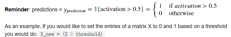
Exercise 9 predict

Predict with your model by building predict(). Use forward propagation to predict results.

# GRADED FUNCTION: predict

def predict(parameters, X):
    """
    Using the learned parameters, predicts a class for each example in X
    
    Arguments:
    parameters -- python dictionary containing your parameters 
    X -- input data of size (n_x, m)
    
    Returns
    predictions -- vector of predictions of our model (red: 0 / blue: 1)
    """
    
    # Computes probabilities using forward propagation, and classifies to 0/1 using 0.5 as the threshold.
    #(≈ 2 lines of code)
    # A2, cache = ...
    # predictions = ...
    # YOUR CODE STARTS HERE
    A2, cache = forward_propagation(X, parameters)
    predictions = (A2>0.5)
    
    # YOUR CODE ENDS HERE
    
    return predictions

这里prediction的结果必须如上图所示，即使你放在array中，这里也能通过测试，但是后续测试模型会出错