信号峰拟合的MATLAB程序，包括高斯拟合，多高斯拟合等多种类型

最新推荐文章于 2024-05-06 11:28:35 发布

交大之心

最新推荐文章于 2024-05-06 11:28:35 发布

阅读量1.2w

点赞数 5

分类专栏：学习

学习专栏收录该内容

21 篇文章 0 订阅

订阅专栏

今天准备弄双高斯拟合，看到一个信号峰拟合的MATLAB版本的程序，大体看了一下，很不错，先MARK一下，以后再详细研究。

http://terpconnect.umd.edu/~toh/spectrum/CurveFittingC.html

http://terpconnect.umd.edu/~toh/spectrum/InteractivePeakFitter.htm

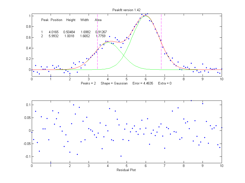
下面是其CODE。感叹别人的代码写的那个结构可扩展性，牛人啊！先来看他的一个双高斯拟合示例：

下面是MATLAB峰拟合函数：

[plain] view plain copy

print ?

function [FitResults,LowestError,BestStart,xi,yi]=peakfit(signal,center,window,NumPeaks,peakshape,extra,NumTrials,start,AUTOZERO)
% Version 2.2: October, 2011. Adds exponential pulse and sigmoid models
% A command-line peak fitting program for time-series signals,
% written as a self-contained Matlab function in a single m-file.
% Uses an non-linear optimization algorithm to decompose a complex,
% overlapping-peak signal into its component parts. The objective
% is to determine whether your signal can be represented as the sum of
% fundamental underlying peaks shapes. Accepts signals of any length,
% including those with non-integer and non-uniform x-values. Fits
% Gaussian, equal-width Gaussians, exponentially-broadened Gaussian,
% Lorentzian, equal-width Lorentzians, Pearson, Logistic, exponential
% pulse, abd sigmoid shapes (expandable to other shapes). This is a command
% line version, usable from a remote terminal. It is capable of making
% multiple trial fits with sightly different starting values and taking
% the one with the lowest mean fit error. Version 2.2: Sept, 2011.
%
% PEAKFIT(signal);
% Performs an iterative least-squares fit of a single Gaussian
% peak to the data matrix "signal", which has x values
% in column 1 and Y values in column 2 (e.g. [x y])
%
% PEAKFIT(signal,center,window);
% Fits a single Gaussian peak to a portion of the
% matrix "signal". The portion is centered on the
% x-value "center" and has width "window" (in x units).
%
% PEAKFIT(signal,center,window,NumPeaks);
% "NumPeaks" = number of peaks in the model (default is 1 if not
% specified).
%
% PEAKFIT(signal,center,window,NumPeaks,peakshape);
% Specifies the peak shape of the model: "peakshape" = 1-5.
% (1=Gaussian (default), 2=Lorentzian, 3=logistic, 4=Pearson,
% 5=exponentionally broadened Gaussian; 6=equal-width Gaussians;
% 7=Equal-width Lorentzians; 8=exponentionally broadened equal-width
% Gaussian, 9=exponential pulse, 10=sigmoid).
%
% PEAKFIT(signal,center,window,NumPeaks,peakshape,extra)
% Specifies the value of 'extra', used in the Pearson and the
% exponentionally broadened Gaussian shapes to fine-tune the peak shape.
%
% PEAKFIT(signal,center,window,NumPeaks,peakshape,extra,NumTrials);
% Performs "NumTrials" trial fits and selects the best one (with lowest
% fitting error). NumTrials can be any positive integer (default is 1).
%
% PEAKFIT(signal,center,window,NumPeaks,peakshape,extra,NumTrials,start)
% Specifies the first guesses vector "firstguess" for the peak positions
% and widths, e.g. start=[position1 width1 position2 width2 ...]
%
% [FitResults,MeanFitError]=PEAKFIT(signal,center,window...)
% Returns the FitResults vector in the order peak number, peak
% position, peak height, peak width, and peak area), and the MeanFitError
% (the percent RMS difference between the data and the model in the
% selected segment of that data) of the best fit.
%
% Optional output parameters
% 1. FitResults: a table of model peak parameters, one row for each peak,
% listing Peak number, Peak position, Height, Width, and Peak area.
% 2. LowestError: The rms fitting error of the best trial fit.
% 3. BestStart: the starting guesses that gave the best fit.
% 4. xi: vector containing 100 interploated x-values for the model peaks.
% 5. yi: matrix containing the y values of each model peak at each xi.
% Type plot(xi,yi(1,:)) to plot peak 1 or plot(xi,yi) to plot all peaks
%
% T. C. O'Haver (toh@umd.edu). Version 2.2
%
% Example 1:
% >> x=[0:.1:10]';y=exp(-(x-5).^2);peakfit([x y])
% Fits exp(-x)^2 with a single Gaussian peak model.
%
% Peak number Peak position Height Width Peak area
% 1 5 1 1.665 1.7725
%
% Example 2:
% x=[0:.1:10]';y=exp(-(x-5).^2)+.1*randn(size(x));peakfit([x y])
% Like Example 1, except that random noise is added to the y data.
% ans =
% 1 5.0279 0.9272 1.7948 1.7716
%
% Example 3:
% x=[0:.1:10];y=exp(-(x-5).^2)+.5*exp(-(x-3).^2)+.1*randn(size(x));
% peakfit([x' y'],5,19,2,1,0,1)
% Fits a noisy two-peak signal with a double Gaussian model (NumPeaks=2).
% ans =
% 1 3.0001 0.49489 1.642 0.86504
% 2 4.9927 1.0016 1.6597 1.7696
%
% Example 4:
% >> y=lorentzian(1:100,50,2);peakfit(y,50,100,1,2)
% Create and fit Lorentzian located at x=50, height=1, width=2.
% ans =
% 1 50 0.99974 1.9971 3.1079
% Example 5:
% >> x=[0:.005:1];y=humps(x);peakfit([x' y'],.3,.7,1,4,3);
% Fits a portion of the humps function, 0.7 units wide and centered on
% x=0.3, with a single (NumPeaks=1) Pearson function (peakshape=4)
% with extra=3 (controls shape of Pearson function).
%
% Example 6:
% >> x=[0:.005:1];y=(humps(x)+humps(x-.13)).^3;smatrix=[x' y'];
% >> [FitResults,MeanFitError]=peakfit(smatrix,.4,.7,2,1,0,10)
% Creates a data matrix 'smatrix', fits a portion to a two-peak Gaussian
% model, takes the best of 10 trials. Returns FitResults and MeanFitError.
% FitResults =
% 1 0.31056 2.0125e+006 0.11057 2.3689e+005
% 2 0.41529 2.2403e+006 0.12033 2.8696e+005
% MeanFitError =
% 1.1899
%
% Example 7:
% >> peakfit([x' y'],.4,.7,2,1,0,10,[.3 .1 .5 .1]);
% As above, but specifies the first-guess position and width of the two
% peaks, in the order [position1 width1 position2 width2]
%
% Example 8:
% >> peakfit([x' y'],.4,.7,2,1,0,10,[.3 .1 .5 .1],0);
% As above, but sets AUTOZERO mode in the last argument.
% AUROZERO=0 does not subtract baseline from data segment.
% AUROZERO=1 (default) subtracts linear baseline from data segment.
% AUROZERO=2, subtracts quadratic baseline from data segment.
%
% For more details, see
% http://terpconnect.umd.edu/~toh/spectrum/CurveFittingC.html and
% http://terpconnect.umd.edu/~toh/spectrum/InteractivePeakFitter.htm
%
global AA xxx PEAKHEIGHTS
format short g
format compact
warning off all
datasize=size(signal);
if datasize(1)<datasize(2),signal=signal';end
datasize=size(signal);
if datasize(2)==1, % Must be isignal(Y-vector)
X=1:length(signal); % Create an independent variable vector
Y=signal;
else
% Must be isignal(DataMatrix)
X=signal(:,1); % Split matrix argument
Y=signal(:,2);
end
X=reshape(X,1,length(X)); % Adjust X and Y vector shape to 1 x n (rather than n x 1)
Y=reshape(Y,1,length(Y));
% If necessary, flip the data vectors so that X increases
if X(1)>X(length(X)),
disp('X-axis flipped.')
X=fliplr(X);
Y=fliplr(Y);
end
% Y=Y-min(Y); % Remove excess offset from data
% Isolate desired segment from data set for curve fitting
if nargin==1 || nargin==2,center=(max(X)-min(X))/2;window=max(X)-min(X);end
xoffset=center-window/2;
n1=val2ind(X,center-window/2);
n2=val2ind(X,center+window/2);
if window==0,n1=1;n2=length(X);end
xx=X(n1:n2)-xoffset;
yy=Y(n1:n2);
ShapeString='Gaussian';
% Define values of any missing arguments
switch nargin
case 1
NumPeaks=1;
peakshape=1;
extra=0;
NumTrials=1;
xx=X;yy=Y;
start=calcstart(xx,NumPeaks,xoffset);
AUTOZERO=1;
case 2
NumPeaks=1;
peakshape=1;
extra=0;
NumTrials=1;
xx=signal;yy=center;
start=calcstart(xx,NumPeaks,xoffset);
AUTOZERO=1;
case 3
NumPeaks=1;
peakshape=1;
extra=0;
NumTrials=1;
start=calcstart(xx,NumPeaks,xoffset);
AUTOZERO=1;
case 4
peakshape=1;
extra=0;
NumTrials=1;
start=calcstart(xx,NumPeaks,xoffset);
AUTOZERO=1;
case 5
extra=0;
NumTrials=1;
start=calcstart(xx,NumPeaks,xoffset);
AUTOZERO=1;
case 6
NumTrials=1;
start=calcstart(xx,NumPeaks,xoffset);
AUTOZERO=1;
case 7
start=calcstart(xx,NumPeaks,xoffset);
AUTOZERO=1;
case 8
AUTOZERO=1;
otherwise
end % switch nargin
% Remove baseline from data segment (alternative code)
% lxx=length(xx);
% bkgsize=10;
% if AUTOZERO==1, % linear autozero operation
% XX1=xx(1:round(lxx/bkgsize));
% XX2=xx((lxx-round(lxx/bkgsize)):lxx);
% Y1=yy(1:round(length(xx)/bkgsize));
% Y2=yy((lxx-round(lxx/bkgsize)):lxx);
% bkgcoef=polyfit([XX1,XX2],[Y1,Y2],1); % Fit straight line to sub-group of points
% bkg=polyval(bkgcoef,xx);
% yy=yy-bkg;
% end % if
% Remove baseline from data segment
X1=min(xx);X2=max(xx);Y1=min(Y);Y2=max(Y);
if AUTOZERO==1, % linear autozero operation
Y1=mean(yy(1:length(xx)/20));
Y2=mean(yy((length(xx)-length(xx)/20):length(xx)));
yy=yy-((Y2-Y1)/(X2-X1)*(xx-X1)+Y1);
end % if
if AUTOZERO==2, % Quadratic autozero operation
XX1=xx(1:round(lxx/bkgsize));
XX2=xx((lxx-round(lxx/bkgsize)):lxx);
Y1=yy(1:round(length(xx)/bkgsize));
Y2=yy((lxx-round(lxx/bkgsize)):lxx);
bkgcoef=polyfit([XX1,XX2],[Y1,Y2],2); % Fit parabola to sub-group of points
bkg=polyval(bkgcoef,xx);
yy=yy-bkg;
end % if autozero
PEAKHEIGHTS=zeros(1,NumPeaks);
n=length(xx);
newstart=start;
switch NumPeaks
case 1
newstart(1)=start(1)-xoffset;
case 2
newstart(1)=start(1)-xoffset;
newstart(3)=start(3)-xoffset;
case 3
newstart(1)=start(1)-xoffset;
newstart(3)=start(3)-xoffset;
newstart(5)=start(5)-xoffset;
case 4
newstart(1)=start(1)-xoffset;
newstart(3)=start(3)-xoffset;
newstart(5)=start(5)-xoffset;
newstart(7)=start(7)-xoffset;
case 5
newstart(1)=start(1)-xoffset;
newstart(3)=start(3)-xoffset;
newstart(5)=start(5)-xoffset;
newstart(7)=start(7)-xoffset;
newstart(9)=start(9)-xoffset;
case 6
newstart(1)=start(1)-xoffset;
newstart(3)=start(3)-xoffset;
newstart(5)=start(5)-xoffset;
newstart(7)=start(7)-xoffset;
newstart(9)=start(9)-xoffset;
newstart(11)=start(11)-xoffset;
otherwise
end % switch NumPeaks
% Perform peak fitting for selected peak shape using fminsearch function
options = optimset('TolX',.00001,'Display','off' );
LowestError=1000; % or any big number greater than largest error expected
FitParameters=zeros(1,NumPeaks.*2);
BestStart=zeros(1,NumPeaks.*2);
height=zeros(1,NumPeaks);
bestmodel=zeros(size(yy));
for k=1:NumTrials,
% disp(['Trial number ' num2str(k) ] ) % optionally prints the current trial number as progress indicator
switch peakshape
case 1
TrialParameters=fminsearch(@fitgaussian,newstart,options,xx,yy);
ShapeString='Gaussian';
case 2
TrialParameters=fminsearch(@fitlorentzian,newstart,options,xx,yy);
ShapeString='Lorentzian';
case 3
TrialParameters=fminsearch(@fitlogistic,newstart,options,xx,yy);
ShapeString='Logistic';
case 4
TrialParameters=fminsearch(@fitpearson,newstart,options,xx,yy,extra);
ShapeString='Pearson';
case 5
TrialParameters=fminsearch(@fitexpgaussian,newstart,options,xx,yy,-extra);
ShapeString='ExpGaussian';
case 6
cwnewstart(1)=newstart(1);
for pc=2:NumPeaks,
cwnewstart(pc)=newstart(2.*pc-1);
end
cwnewstart(NumPeaks+1)=(max(xx)-min(xx))/5;
TrialParameters=fminsearch(@fitewgaussian,cwnewstart,options,xx,yy);
ShapeString='Equal width Gaussians';
case 7
cwnewstart(1)=newstart(1);
for pc=2:NumPeaks,
cwnewstart(pc)=newstart(2.*pc-1);
end
cwnewstart(NumPeaks+1)=(max(xx)-min(xx))/5;
TrialParameters=fminsearch(@fitlorentziancw,cwnewstart,options,xx,yy);
ShapeString='Equal width Lorentzians';
case 8
cwnewstart(1)=newstart(1);
for pc=2:NumPeaks,
cwnewstart(pc)=newstart(2.*pc-1);
end
cwnewstart(NumPeaks+1)=(max(xx)-min(xx))/5;
TrialParameters=fminsearch(@fitexpewgaussian,cwnewstart,options,xx,yy,-extra);
ShapeString='Exp. equal width Gaussians';
case 9
TrialParameters=fminsearch(@fitexppulse,newstart,options,xx,yy);
ShapeString='Exponential Pulse';
case 10
TrialParameters=fminsearch(@fitsigmoid,newstart,options,xx,yy);
ShapeString='Sigmoid';
otherwise
end % switch peakshape
% Construct model from Trial parameters
A=zeros(NumPeaks,n);
for m=1:NumPeaks,
switch peakshape
case 1
A(m,:)=gaussian(xx,TrialParameters(2*m-1),TrialParameters(2*m));
case 2
A(m,:)=lorentzian(xx,TrialParameters(2*m-1),TrialParameters(2*m));
case 3
A(m,:)=logistic(xx,TrialParameters(2*m-1),TrialParameters(2*m));
case 4
A(m,:)=pearson(xx,TrialParameters(2*m-1),TrialParameters(2*m),extra);
case 5
A(m,:)=expgaussian(xx,TrialParameters(2*m-1),TrialParameters(2*m),-extra)';
case 6
A(m,:)=gaussian(xx,TrialParameters(m),TrialParameters(NumPeaks+1));
case 7
A(m,:)=lorentzian(xx,TrialParameters(m),TrialParameters(NumPeaks+1));
case 8
A(m,:)=expgaussian(xx,TrialParameters(m),TrialParameters(NumPeaks+1),-extra)';
case 9
A(m,:)=exppulse(xx,TrialParameters(2*m-1),TrialParameters(2*m));
case 10
A(m,:)=sigmoid(xx,TrialParameters(2*m-1),TrialParameters(2*m));
otherwise
end % switch
switch NumPeaks % adds random variation to non-linear parameters
case 1
newstart=[newstart(1)*(1+randn/50) newstart(2)*(1+randn/10)];
case 2
newstart=[newstart(1)*(1+randn/50) newstart(2)*(1+randn/10) newstart(3)*(1+randn/50) newstart(4)*(1+randn/10)];
case 3
newstart=[newstart(1)*(1+randn/50) newstart(2)*(1+randn/10) newstart(3)*(1+randn/50) newstart(4)*(1+randn/10) newstart(5)*(1+randn/50) newstart(6)*(1+randn/10)];
case 4
newstart=[newstart(1)*(1+randn/50) newstart(2)*(1+randn/10) newstart(3)*(1+randn/50) newstart(4)*(1+randn/10) newstart(5)*(1+randn/50) newstart(6)*(1+randn/10) newstart(7)*(1+randn/50) newstart(8)*(1+randn/10)];
case 5
newstart=[newstart(1)*(1+randn/50) newstart(2)*(1+randn/10) newstart(3)*(1+randn/50) newstart(4)*(1+randn/10) newstart(5)*(1+randn/50) newstart(6)*(1+randn/10) newstart(7)*(1+randn/50) newstart(8)*(1+randn/10) newstart(9)*(1+randn/50) newstart(10)*(1+randn/10)];
otherwise
end % switch NumPeaks
end % for
% Multiplies each row by the corresponding amplitude and adds them up
model=PEAKHEIGHTS'*A;
% Compare trial model to data segment and compute the fit error
MeanFitError=100*norm(yy-model)./(sqrt(n)*max(yy));
% Take only the single fit that has the lowest MeanFitError
if MeanFitError<LowestError,
if min(PEAKHEIGHTS)>0, % Consider only fits with positive peak heights
LowestError=MeanFitError; % Assign LowestError to the lowest MeanFitError
FitParameters=TrialParameters; % Assign FitParameters to the fit with the lowest MeanFitError
BestStart=newstart; % Assign BestStart to the start with the lowest MeanFitError
height=PEAKHEIGHTS; % Assign height to the PEAKHEIGHTS with the lowest MeanFitError
bestmodel=model; % Assign bestmodel to the model with the lowest MeanFitError
end % if min(PEAKHEIGHTS)>0
end % if MeanFitError<LowestError
end % for k (NumTrials)
%
% Construct model from best-fit parameters
AA=zeros(NumPeaks,100);
xxx=linspace(min(xx),max(xx));
for m=1:NumPeaks,
switch peakshape
case 1
AA(m,:)=gaussian(xxx,FitParameters(2*m-1),FitParameters(2*m));
case 2
AA(m,:)=lorentzian(xxx,FitParameters(2*m-1),FitParameters(2*m));
case 3
AA(m,:)=logistic(xxx,FitParameters(2*m-1),FitParameters(2*m));
case 4
AA(m,:)=pearson(xxx,FitParameters(2*m-1),FitParameters(2*m),extra);
case 5
AA(m,:)=expgaussian(xxx,FitParameters(2*m-1),FitParameters(2*m),-extra*length(xxx)./length(xx))';
case 6
AA(m,:)=gaussian(xxx,FitParameters(m),FitParameters(NumPeaks+1));
case 7
AA(m,:)=lorentzian(xxx,FitParameters(m),FitParameters(NumPeaks+1));
case 8
AA(m,:)=expgaussian(xxx,FitParameters(m),FitParameters(NumPeaks+1),-extra*length(xxx)./length(xx))';
case 9
AA(m,:)=exppulse(xxx,FitParameters(2*m-1),FitParameters(2*m));
case 10
AA(m,:)=sigmoid(xxx,FitParameters(2*m-1),FitParameters(2*m));
otherwise
end % switch
end % for
% Multiplies each row by the corresponding amplitude and adds them up
heightsize=size(height');
AAsize=size(AA);
if heightsize(2)==AAsize(1),
mmodel=height'*AA;
else
mmodel=height*AA;
end
% Top half of the figure shows original signal and the fitted model.
subplot(2,1,1);plot(xx+xoffset,yy,'b.'); % Plot the original signal in blue dots
hold on
for m=1:NumPeaks,
plot(xxx+xoffset,height(m)*AA(m,:),'g') % Plot the individual component peaks in green lines
area(m)=trapz(xxx+xoffset,height(m)*AA(m,:)); % Compute the area of each component peak using trapezoidal method
yi(m,:)=height(m)*AA(m,:); % (NEW) Place y values of individual model peaks into matrix yi
end
xi=xxx+xoffset; % (NEW) Place the x-values of the individual model peaks into xi
% Mark starting peak positions with vertical dashed lines
for marker=1:NumPeaks,
markx=BestStart((2*marker)-1);
subplot(2,1,1);plot([markx+xoffset markx+xoffset],[0 max(yy)],'m--')
end % for
plot(xxx+xoffset,mmodel,'r'); % Plot the total model (sum of component peaks) in red lines
hold off;
axis([min(xx)+xoffset max(xx)+xoffset min(yy) max(yy)]);
switch AUTOZERO,
case 0
title('Peakfit 2.2. Autozero OFF.')
case 1
title('Peakfit 2.2. Linear autozero.')
case 2
title('Peakfit 2.2. Quadratic autozero.')
end
if peakshape==4||peakshape==5||peakshape==8, % Shapes with Extra factor
xlabel(['Peaks = ' num2str(NumPeaks) ' Shape = ' ShapeString ' Error = ' num2str(round(100*LowestError)/100) '% Extra = ' num2str(extra) ] )
else
xlabel(['Peaks = ' num2str(NumPeaks) ' Shape = ' ShapeString ' Error = ' num2str(round(100*LowestError)/100) '%' ] )
end
% Bottom half of the figure shows the residuals and displays RMS error
% between original signal and model
residual=yy-bestmodel;
subplot(2,1,2);plot(xx+xoffset,residual,'b.')
axis([min(xx)+xoffset max(xx)+xoffset min(residual) max(residual)]);
xlabel('Residual Plot')
% Put results into a matrix, one row for each peak, showing peak index number,
% position, amplitude, and width.
for m=1:NumPeaks,
if m==1,
if peakshape==6||peakshape==7||peakshape==8, % equal-width peak models
FitResults=[[round(m) FitParameters(m)+xoffset height(m) abs(FitParameters(NumPeaks+1)) area(m)]];
else
FitResults=[[round(m) FitParameters(2*m-1)+xoffset height(m) abs(FitParameters(2*m)) area(m)]];
end % if peakshape
else
if peakshape==6||peakshape==7||peakshape==8, % equal-width peak models
FitResults=[FitResults ; [round(m) FitParameters(m)+xoffset height(m) abs(FitParameters(NumPeaks+1)) area(m)]];
else
FitResults=[FitResults ; [round(m) FitParameters(2*m-1)+xoffset height(m) abs(FitParameters(2*m)) area(m)]];
end % if peakshape
end % m==1
end % for m=1:NumPeaks
% Display Fit Results on upper graph
subplot(2,1,1);
startx=min(xx)+xoffset+(max(xx)-min(xx))./20;
dxx=(max(xx)-min(xx))./10;
dyy=(max(yy)-min(yy))./10;
starty=max(yy)-dyy;
FigureSize=get(gcf,'Position');
if peakshape==9||peakshape==10,
text(startx,starty+dyy/2,['Peak # tau1 Height tau2 Area'] );
else
text(startx,starty+dyy/2,['Peak # Position Height Width Area'] );
end
% Display FitResults using sprintf
for peaknumber=1:NumPeaks,
for column=1:5,
itemstring=sprintf('%0.4g',FitResults(peaknumber,column));
xposition=startx+(1.7.*dxx.*(column-1).*(600./FigureSize(3)));
yposition=starty-peaknumber.*dyy.*(400./FigureSize(4));
text(xposition,yposition,itemstring);
end
end
% ----------------------------------------------------------------------
function start=calcstart(xx,NumPeaks,xoffset)
n=max(xx)-min(xx);
start=[];
startpos=[n/(NumPeaks+1):n/(NumPeaks+1):n-(n/(NumPeaks+1))]+min(xx);
for marker=1:NumPeaks,
markx=startpos(marker)+ xoffset;
start=[start markx n/5];
end % for marker
% ----------------------------------------------------------------------
function [index,closestval]=val2ind(x,val)
% Returns the index and the value of the element of vector x that is closest to val
% If more than one element is equally close, returns vectors of indicies and values
% Tom O'Haver (toh@umd.edu) October 2006
% Examples: If x=[1 2 4 3 5 9 6 4 5 3 1], then val2ind(x,6)=7 and val2ind(x,5.1)=[5 9]
% [indices values]=val2ind(x,3.3) returns indices = [4 10] and values = [3 3]
dif=abs(x-val);
index=find((dif-min(dif))==0);
closestval=x(index);
% ----------------------------------------------------------------------
function err = fitgaussian(lambda,t,y)
% Fitting function for a Gaussian band signal.
global PEAKHEIGHTS
numpeaks=round(length(lambda)/2);
A = zeros(length(t),numpeaks);
for j = 1:numpeaks,
A(:,j) = gaussian(t,lambda(2*j-1),lambda(2*j))';
end
PEAKHEIGHTS = abs(A\y');
z = A*PEAKHEIGHTS;
err = norm(z-y');
% ----------------------------------------------------------------------
function err = fitewgaussian(lambda,t,y)
% Fitting function for a Gaussian band signal with equal peak widths.
global PEAKHEIGHTS
numpeaks=round(length(lambda)-1);
A = zeros(length(t),numpeaks);
for j = 1:numpeaks,
A(:,j) = gaussian(t,lambda(j),lambda(numpeaks+1))';
end
PEAKHEIGHTS = abs(A\y');
z = A*PEAKHEIGHTS;
err = norm(z-y');
% ----------------------------------------------------------------------
function err = fitgaussianfw(lambda,t,y)
% Fitting function for a Gaussian band signal with fixed peak widths.
global PEAKHEIGHTS
numpeaks=round(length(lambda)-1);
A = zeros(length(t),numpeaks);
for j = 1:numpeaks,
A(:,j) = gaussian(t,lambda(j),lambda(numpeaks+1))';
end
PEAKHEIGHTS = abs(A\y');
z = A*PEAKHEIGHTS;
err = norm(z-y');
% ----------------------------------------------------------------------
function err = fitlorentziancw(lambda,t,y)
% Fitting function for a Lorentzian band signal with equal peak widths.
global PEAKHEIGHTS
numpeaks=round(length(lambda)-1);
A = zeros(length(t),numpeaks);
for j = 1:numpeaks,
A(:,j) = lorentzian(t,lambda(j),lambda(numpeaks+1))';
end
PEAKHEIGHTS = abs(A\y');
z = A*PEAKHEIGHTS;
err = norm(z-y');
% ----------------------------------------------------------------------
function g = gaussian(x,pos,wid)
% gaussian(X,pos,wid) = gaussian peak centered on pos, half-width=wid
% X may be scalar, vector, or matrix, pos and wid both scalar
% Examples: gaussian([0 1 2],1,2) gives result [0.5000 1.0000 0.5000]
% plot(gaussian([1:100],50,20)) displays gaussian band centered at 50 with width 20.
g = exp(-((x-pos)./(0.6005615.*wid)) .^2);
% ----------------------------------------------------------------------
function err = fitlorentzian(lambda,t,y)
% Fitting function for single lorentzian, lambda(1)=position, lambda(2)=width
% Fitgauss assumes a lorentzian function
global PEAKHEIGHTS
A = zeros(length(t),round(length(lambda)/2));
for j = 1:length(lambda)/2,
A(:,j) = lorentzian(t,lambda(2*j-1),lambda(2*j))';
end
PEAKHEIGHTS = A\y';
z = A*PEAKHEIGHTS;
err = norm(z-y');
% ----------------------------------------------------------------------
function g = lorentzian(x,position,width)
% lorentzian(x,position,width) Lorentzian function.
% where x may be scalar, vector, or matrix
% position and width scalar
% T. C. O'Haver, 1988
% Example: lorentzian([1 2 3],2,2) gives result [0.5 1 0.5]
g=ones(size(x))./(1+((x-position)./(0.5.*width)).^2);
% ----------------------------------------------------------------------
function err = fitlogistic(lambda,t,y)
% Fitting function for logistic, lambda(1)=position, lambda(2)=width
% between the data and the values computed by the current
% function of lambda. Fitlogistic assumes a logistic function
% T. C. O'Haver, May 2006
global PEAKHEIGHTS
A = zeros(length(t),round(length(lambda)/2));
for j = 1:length(lambda)/2,
A(:,j) = logistic(t,lambda(2*j-1),lambda(2*j))';
end
PEAKHEIGHTS = A\y';
z = A*PEAKHEIGHTS;
err = norm(z-y');
% ----------------------------------------------------------------------
function g = logistic(x,pos,wid)
% logistic function. pos=position; wid=half-width (both scalar)
% logistic(x,pos,wid), where x may be scalar, vector, or matrix
% pos=position; wid=half-width (both scalar)
% T. C. O'Haver, 1991
n = exp(-((x-pos)/(.477.*wid)) .^2);
g = (2.*n)./(1+n);
% ----------------------------------------------------------------------
function err = fitlognormal(lambda,t,y)
% Fitting function for lognormal, lambda(1)=position, lambda(2)=width
% between the data and the values computed by the current
% function of lambda. Fitlognormal assumes a lognormal function
% T. C. O'Haver, May 2006
global PEAKHEIGHTS
A = zeros(length(t),round(length(lambda)/2));
for j = 1:length(lambda)/2,
A(:,j) = lognormal(t,lambda(2*j-1),lambda(2*j))';
end
PEAKHEIGHTS = A\y';
z = A*PEAKHEIGHTS;
err = norm(z-y');
% ----------------------------------------------------------------------
function g = lognormal(x,pos,wid)
% lognormal function. pos=position; wid=half-width (both scalar)
% lognormal(x,pos,wid), where x may be scalar, vector, or matrix
% pos=position; wid=half-width (both scalar)
% T. C. O'Haver, 1991
g = exp(-(log(x/pos)/(0.01.*wid)) .^2);
% ----------------------------------------------------------------------
function err = fitpearson(lambda,t,y,shapeconstant)
% Fitting functions for a Pearson 7 band signal.
% T. C. O'Haver (toh@umd.edu), Version 1.3, October 23, 2006.
global PEAKHEIGHTS
A = zeros(length(t),round(length(lambda)/2));
for j = 1:length(lambda)/2,
A(:,j) = pearson(t,lambda(2*j-1),lambda(2*j),shapeconstant)';
end
PEAKHEIGHTS = A\y';
z = A*PEAKHEIGHTS;
err = norm(z-y');
% ----------------------------------------------------------------------
function g = pearson(x,pos,wid,m)
% Pearson VII function.
% g = pearson7(x,pos,wid,m) where x may be scalar, vector, or matrix
% pos=position; wid=half-width (both scalar)
% m=some number
% T. C. O'Haver, 1990
g=ones(size(x))./(1+((x-pos)./((0.5.^(2/m)).*wid)).^2).^m;
% ----------------------------------------------------------------------
function err = fitexpgaussian(lambda,t,y,timeconstant)
% Fitting functions for a exponentially-broadened Gaussian band signal.
% T. C. O'Haver, October 23, 2006.
global PEAKHEIGHTS
A = zeros(length(t),round(length(lambda)/2));
for j = 1:length(lambda)/2,
A(:,j) = expgaussian(t,lambda(2*j-1),lambda(2*j),timeconstant);
end
PEAKHEIGHTS = A\y';
z = A*PEAKHEIGHTS;
err = norm(z-y');
% ----------------------------------------------------------------------
function err = fitexpewgaussian(lambda,t,y,timeconstant)
% Fitting function for exponentially-broadened Gaussian bands with equal peak widths.
global PEAKHEIGHTS
numpeaks=round(length(lambda)-1);
A = zeros(length(t),numpeaks);
for j = 1:numpeaks,
A(:,j) = expgaussian(t,lambda(j),lambda(numpeaks+1),timeconstant);
end
PEAKHEIGHTS = abs(A\y');
z = A*PEAKHEIGHTS;
err = norm(z-y');
% ----------------------------------------------------------------------
function g = expgaussian(x,pos,wid,timeconstant)
% Exponentially-broadened gaussian(x,pos,wid) = gaussian peak centered on pos, half-width=wid
% x may be scalar, vector, or matrix, pos and wid both scalar
% T. C. O'Haver, 2006
g = exp(-((x-pos)./(0.6005615.*wid)) .^2);
g = ExpBroaden(g',timeconstant);
% ----------------------------------------------------------------------
function yb = ExpBroaden(y,t)
% ExpBroaden(y,t) convolutes y by an exponential decay of time constant t
% by multiplying Fourier transforms and inverse transforming the result.
fy=fft(y);
a=exp(-[1:length(y)]./t);
fa=fft(a);
fy1=fy.*fa';
yb=real(ifft(fy1))./sum(a);
% ----------------------------------------------------------------------
function err = fitexppulse(tau,x,y)
% Iterative fit of the sum of exponental pulses
% of the form Height.*exp(-tau1.*x).*(1-exp(-tau2.*x)))
global PEAKHEIGHTS
A = zeros(length(x),round(length(tau)/2));
for j = 1:length(tau)/2,
A(:,j) = exppulse(x,tau(2*j-1),tau(2*j));
end
PEAKHEIGHTS =abs(A\y');
z = A*PEAKHEIGHTS;
err = norm(z-y');
% ----------------------------------------------------------------------
function g = exppulse(x,t1,t2)
% Exponential pulse of the form
% Height.*exp(-tau1.*x).*(1-exp(-tau2.*x)))
e=(x-t1)./t2;
p = 4*exp(-e).*(1-exp(-e));
p=p .* [p>0];
g = p';
% ----------------------------------------------------------------------
function err = fitsigmoid(tau,x,y)
% Fitting function for iterative fit to the sum of
% sigmiods of the form Height./(1 + exp((t1 - t)/t2))
global PEAKHEIGHTS
A = zeros(length(x),round(length(tau)/2));
for j = 1:length(tau)/2,
A(:,j) = sigmoid(x,tau(2*j-1),tau(2*j));
end
PEAKHEIGHTS = A\y';
z = A*PEAKHEIGHTS;
err = norm(z-y');
% ----------------------------------------------------------------------
function g=sigmoid(x,t1,t2)
g=1./(1 + exp((t1 - x)./t2))';

交大之心

关注

5
点赞
踩
50

收藏

觉得还不错? 一键收藏
2
评论
信号峰拟合的MATLAB程序，包括高斯拟合，多高斯拟合等多种类型

今天准备弄双高斯拟合，看到一个信号峰拟合的MATLAB版本的程序，大体看了一下，很不错，先MARK一下，以后再详细研究。 http://terpconnect.umd.edu/~toh/spectrum/CurveFittingC.htmlhttp://terpconnect.umd.edu/~toh/spectrum/InteractivePeakFitter.htm 下面是其
复制链接

扫一扫