高斯回归拟合x与y数据,自定义置信区间及MATLAB代码解析,简洁易用的案例分析

高斯回归拟合x与y,带置信区间
置信区间可自定义
根据案例数据准备自己的自变量x与因变量y数据
按照相应格式替换为自己数据即可
MATLAB代码,备注清晰,易于使用

ID:2360705344962194

Matlab编程


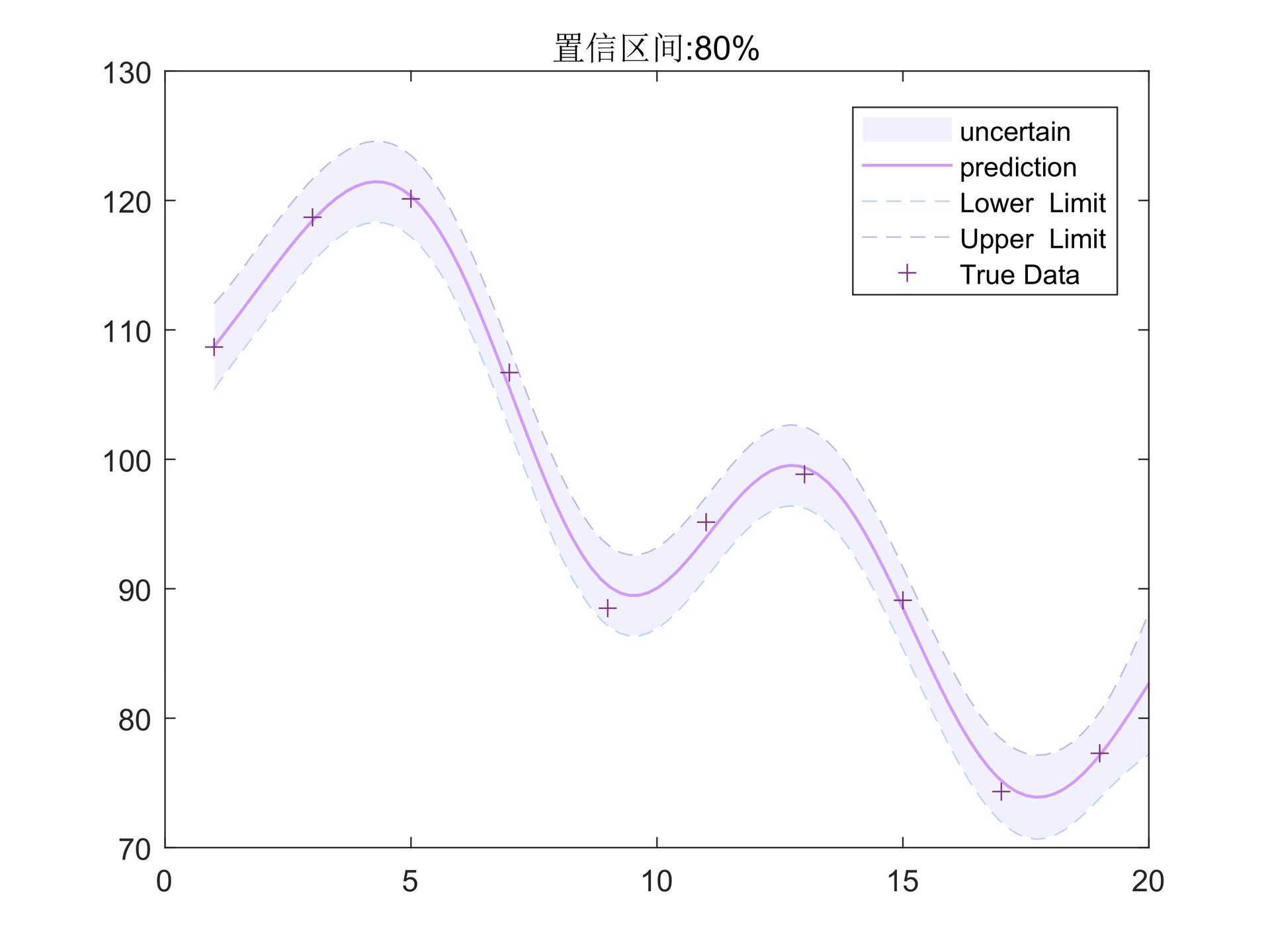
高斯回归拟合是一种常用的统计分析方法,用于研究变量之间的关系和预测未知值。在这篇文章中,我们将重点介绍如何使用高斯回归拟合来分析自变量x与因变量y之间的关系,并给出带置信区间的可自定义示例。

首先,我们需要准备自己的自变量x与因变量y的数据。通过收集与我们研究主题相关的实际案例数据,我们可以获得具有一定代表性的数据样本。这些数据样本可以是实验数据、市场调研数据等,关键是确保数据的准确性和可靠性。

接下来,我们将使用MATLAB代码来进行高斯回归拟合并生成置信区间。MATLAB是一种功能强大的数值计算和科学分析工具,在统计分析中广泛使用。我们的代码将包括数据导入、高斯回归拟合、置信区间计算和结果可视化等步骤。

在代码中,我们将根据相应格式替换自己的数据。通过替换自变量x和因变量y的数据,我们可以将代码应用于我们的具体研究场景,并得到相应的结果。同时,为了使代码易于理解和使用,我们将为每个步骤添加清晰的注释,以提供必要的说明和指导。

在使用代码时&#

  • 6
    点赞
  • 4
    收藏
    觉得还不错? 一键收藏
  • 0
    评论
% This folder contains a collection of "fitting" functions. % (Some has demo options - the third section) % The GENERAL input to the functions should be samples of the distribution. % % for example, if we are to fit a normal distribution ('gaussian') with a mean "u" and varaince "sig"^2 % then the samples will distribute like: % samples = randn(1,10000)*sig + u % %fitting with Least-Squares is done on the histogram of the samples. % fitting with Maximum likelihood is done directly on the samples. % % % Contents of this folder % ======================= % 1) Maximum likelihood estimators % 2) Least squares estimators % 3) EM algorithm for estimation of multivariant gaussian distribution (mixed gaussians) % 4) added folders: Create - which create samples for the EM algorithm test % Plot - used to plot each of the distributions (parametric plot) % % % % % % Maximum likelihood estimators % ============================= % fit_ML_maxwell - fit maxwellian distribution % fit_ML_rayleigh - fit rayleigh distribution % (which is for example: sqrt(abs(randn)^2+abs(randn)^2)) % fit_ML_laplace - fit laplace distribution % fit_ML_log_normal- fit log-normal distribution % fit_ML_normal - fit normal (gaussian) distribution % % NOTE: all estimators are efficient estimators. for this reason, the distribution % might be written in a different way, for example, the "Rayleigh" distribution % is given with a parameter "s" and not "s^2". % % % least squares estimators % ========================= % fit_maxwell_pdf - fits a given curve of a maxwellian distribution % fit_rayleigh_pdf - fits a given curve of a rayleigh distribution % % NOTE: these fit function are used on a histogram output which is like a sampled % distribution function. the given curve MUST be normalized, since the estimator % is trying to fit a normalized distribution function. % % % % % Multivariant Gaussian distribution % ================================== % for demo of 1
matlab中的高斯过程回归fitrgp函数可以用于预测和建模连续型数据。通过该函数,我们可以训练一个高斯过程回归模型,并使用该模型对未知数据进行预测。在预测过程中,我们还可以根据该模型计算并画出置信区间。 首先,使用fitrgp函数训练一个高斯过程回归模型。该函数需要输入一个矩阵X,包含训练数据的特征值,和一个向量Y,包含对应的目标值。可以使用训练数据集(已知的数据)来拟合这个模型。示例代码如下: ```matlab X = [1; 2; 3; 4; 5]; % 训练数据的特征值 Y = [4; 2; 5; 1; 6]; % 训练数据的目标值 model = fitrgp(X, Y); % 训练高斯过程回归模型 ``` 接下来,我们可以使用该模型对未知数据进行预测。预测时,需要将未知数据的特征值作为输入传递给predict函数,并指定返回置信区间。示例代码如下: ```matlab X_pred = [6; 7; 8]; % 未知数据的特征值 [Y_pred, yci] = predict(model, X_pred, 'Alpha', 0.05); % 预测未知数据,并计算置信区间 disp(Y_pred); % 显示预测结果 disp(yci); % 显示置信区间 ``` 在上述代码中,我们使用predict函数预测了未知数据的目标值Y_pred,并使用"Alpha"参数设置了置信水平为0.05(即95%的置信水平)。预测结果Y_pred表示模型对未知数据的预测值,yci表示预测的置信区间。 最后,我们可以将置信区间可视化,以更直观地展示预测的不确定性。示例代码如下: ```matlab plot(X, Y, 'ro'); % 绘制训练数据的散点图 hold on; plot(X_pred, Y_pred, 'b-'); % 绘制预测结果的曲线 fill([X_pred; flipud(X_pred)], [yci(:, 1); flipud(yci(:, 2))], [0.8 0.8 0.8], 'LineStyle', 'none'); % 绘制置信区间的灰色填充 legend('训练数据', '预测结果', '置信区间'); ``` 上述代码使用plot函数绘制了训练数据的散点图,使用绘制预测结果的曲线,并使用fill函数绘制了置信区间的灰色填充。最后,使用legend函数添加了图例。运行上述代码,即可得到包含预测结果和置信区间的可视化图形。 通过使用fitrgp函数进行高斯过程回归预测,并使用predict函数计算置信区间,再结合可视化,我们可以更全面地认识和分析预测结果的不确定性。
评论
添加红包

请填写红包祝福语或标题

红包个数最小为10个

红包金额最低5元

当前余额3.43前往充值 >
需支付:10.00
成就一亿技术人!
领取后你会自动成为博主和红包主的粉丝 规则
hope_wisdom
发出的红包
实付
使用余额支付
点击重新获取
扫码支付
钱包余额 0

抵扣说明:

1.余额是钱包充值的虚拟货币,按照1:1的比例进行支付金额的抵扣。
2.余额无法直接购买下载,可以购买VIP、付费专栏及课程。

余额充值