


目标检测产生与发展
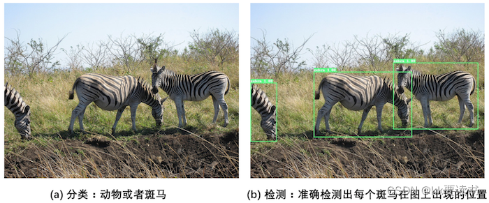
目标检测的主要目的是让计算机可以自动识别图片或者视频帧中所有目标的类别,并在该目标周围绘制边界框,标示出每个目标的位置。如图:
-
物体识别:目标检测的首要任务是识别图像中不同类别的物体。这通常涉及使用深度学习模型,如卷积神经网络(CNN),对图像进行分类,以确定图像中是否存在特定类型的物体。
-
定位物体:与物体识别相结合的是物体定位,即确定图像中物体所在的位置。通常以边界框(bounding box)的形式给出,用矩形框表示物体的位置。
学习了图像分类处理基本流程,我们知道先使用卷积神经网络提取图像特征,然后再用这些特征预测分类概率,最后选出概率最大的类别。但对于目标检测问题,按照这样的流程则行不通。因为在图像分类任务中,对整张图提取特征的过程中没能体现出不同目标之间的区别,最终也就没法分别标示出每个物体所在的位置。为了解决这个问题,结合图片分类任务取得的成功经验,我们可以将目标检测任务进行拆分。假设我们现在有某种方式可以在输入图片上生成一系列可能包含物体的区域,这些区域称为候选区域,在一张图上可以生成很多个候选区域。然后对每个候选区域,可以把它单独当成一幅图像来看待,使用图像分类模型对它进行分类,看它属于哪个类别或者背景(即不包含任何物体的类别)。
目标检测基础概念
边界框(Bounding Box,BBox)
通常使用边界框(bounding box,bbox)来表示物体的位置,边界框是正好能包含物体的矩形框,如图:

有两种格式来表示边界框的位置:
1.xyxy,即(x1,y1,x2,y2),其中(x1,y1)是矩形框左上角的坐标(x2,y2)是矩形框右下角的坐标。
2.xywh,即(x,y,w,h),其中(x,y)是矩形框中心点的坐标,w是矩形框的宽度,ℎh是矩形框的高度。
模型会对目标物体可能出现的位置进行预测,由模型预测出的边界框则称为预测框(prediction box)。要完成一项检测任务,我们通常希望模型能够根据输入的图片,输出一些预测的边界框,以及边界框中所包含的物体的类别或者说属于某个类别的概率,例如这种格式: [L,P,x1,y1,x2,y2],其中L是类别标签,P是物体属于该类别的概率。
锚框(Anchor box)
锚框与物体边界框不同,是由人们假想出来的一种框。先设定好锚框的大小和形状,再以图像上某一个点为中心画出矩形框。示例代码:
# 画图展示如何绘制边界框和锚框
import numpy as np
import matplotlib.pyplot as plt
%matplotlib inline
import matplotlib.patches as patches
from matplotlib.image import imread
import math

# 定义画矩形框的程序
def draw_rectangle(currentAxis, bbox, edgecolor = 'k', facecolor = 'y', fill=False, linestyle='-'):
    # currentAxis,坐标轴,通过plt.gca()获取
    # bbox,边界框,包含四个数值的list, [x1, y1, x2, y2]
    # edgecolor,边框线条颜色
    # facecolor,填充颜色
    # fill, 是否填充
    # linestype,边框线型
    # patches.Rectangle需要传入左上角坐标、矩形区域的宽度、高度等参数
    rect=patches.Rectangle((bbox[0], bbox[1]), bbox[2]-bbox[0]+1, bbox[3]-bbox[1]+1, linewidth=1,
                           edgecolor=edgecolor,facecolor=facecolor,fill=fill, linestyle=linestyle)
    currentAxis.add_patch(rect)


plt.figure(figsize=(10, 10))

filename = '/home/aistudio/work/images/section3/000000086956.jpg'
im = imread(filename)
plt.imshow(im)

# 使用xyxy格式表示物体真实框
bbox1 = [214.29, 325.03, 399.82, 631.37]
bbox2 = [40.93, 141.1, 226.99, 515.73]
bbox3 = [247.2, 131.62, 480.0, 639.32]

currentAxis=plt.gca()

draw_rectangle(currentAxis, bbox1, edgecolor='r')
draw_rectangle(currentAxis, bbox2, edgecolor='r')
draw_rectangle(currentAxis, bbox3,edgecolor='r')

# 绘制锚框
def draw_anchor_box(center, length, scales, ratios, img_height, img_width):
    """
    以center为中心,产生一系列锚框
    其中length指定了一个基准的长度
    scales是包含多种尺寸比例的list
    ratios是包含多种长宽比的list
    img_height和img_width是图片的尺寸,生成的锚框范围不能超出图片尺寸之外
    """
    bboxes = []
    for scale in scales:
        for ratio in ratios:
            h = length*scale*math.sqrt(ratio)
            w = length*scale/math.sqrt(ratio)
            x1 = max(center[0] - w/2., 0.)
            y1 = max(center[1] - h/2., 0.)
            x2 = min(center[0] + w/2. - 1.0, img_width - 1.0)
            y2 = min(center[1] + h/2. - 1.0, img_height - 1.0)
            print(center[0], center[1], w, h)
            bboxes.append([x1, y1, x2, y2])

    for bbox in bboxes:
        draw_rectangle(currentAxis, bbox, edgecolor = 'b')

img_height = im.shape[0]
img_width = im.shape[1]
draw_anchor_box([300., 500.], 100., [2.0], [0.5, 1.0, 2.0], img_height, img_width)


################# 以下为添加文字说明和箭头###############################

plt.text(285, 285, 'G1', color='red', fontsize=20)
plt.arrow(300, 288, 30, 40, color='red', width=0.001, length_includes_head=True, \
         head_width=5, head_length=10, shape='full')

plt.text(190, 320, 'A1', color='blue', fontsize=20)
plt.arrow(200, 320, 30, 40, color='blue', width=0.001, length_includes_head=True, \
         head_width=5, head_length=10, shape='full')

plt.text(160, 370, 'A2', color='blue', fontsize=20)
plt.arrow(170, 370, 30, 40, color='blue', width=0.001, length_includes_head=True, \
         head_width=5, head_length=10, shape='full')

plt.text(115, 420, 'A3', color='blue', fontsize=20)
plt.arrow(127, 420, 30, 40, color='blue', width=0.001, length_includes_head=True, \
         head_width=5, head_length=10, shape='full')

#draw_anchor_box([200., 200.], 100., [2.0], [0.5, 1.0, 2.0])
plt.show()
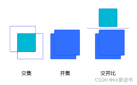
交并比
交并比(Intersection of Union,IoU)这一概念来源于数学中的集合,用来描述两个集合A和B之间的关系,它等于两个集合的交集里面所包含的元素个数,除以它们的并集里面所包含的元素个数,具体计算公式如下:IoU=A∩B/A∪B
假设两个矩形框A和B的位置分别为:
A:[xa1,ya1,xa2,ya2]
B:[xb1,yb1,xb2,yb2]
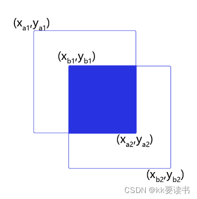
如果二者有相交部分,则相交部分左上角坐标为:
x1=max(xa1,xb1), y1=max(ya1,yb1)
相交部分右下角坐标为:
x2=min(xa2,xb2), y2=min(ya2,yb2)
计算先交部分面积:
intersection=max(x2−x1+1.0,0)⋅max(y2−y1+1.0,0)
矩形框A和B的面积分别是:
SA=(xa2−xa1+1.0)⋅(ya2−ya1+1.0)
SB=(xb2−xb1+1.0)⋅(yb2−yb1+1.0)
计算相并部分面积:
union=SA+SB−intersection
计算交并比:
IoU=intersection/union
# 计算IoU,矩形框的坐标形式为xyxy,这个函数会被保存在box_utils.py文件中
def box_iou_xyxy(box1, box2):
    # 获取box1左上角和右下角的坐标
    x1min, y1min, x1max, y1max = box1[0], box1[1], box1[2], box1[3]
    # 计算box1的面积
    s1 = (y1max - y1min + 1.) * (x1max - x1min + 1.)
    # 获取box2左上角和右下角的坐标
    x2min, y2min, x2max, y2max = box2[0], box2[1], box2[2], box2[3]
    # 计算box2的面积
    s2 = (y2max - y2min + 1.) * (x2max - x2min + 1.)

    # 计算相交矩形框的坐标
    xmin = np.maximum(x1min, x2min)
    ymin = np.maximum(y1min, y2min)
    xmax = np.minimum(x1max, x2max)
    ymax = np.minimum(y1max, y2max)
    # 计算相交矩形行的高度、宽度、面积
    inter_h = np.maximum(ymax - ymin + 1., 0.)
    inter_w = np.maximum(xmax - xmin + 1., 0.)
    intersection = inter_h * inter_w
    # 计算相并面积
    union = s1 + s2 - intersection
    # 计算交并比
    iou = intersection / union
    return iou


bbox1 = [100., 100., 200., 200.]
bbox2 = [120., 120., 220., 220.]
iou = box_iou_xyxy(bbox1, bbox2)
print('IoU is {}'.format(iou))
NMS
在目标检测过程中,网络对同一个目标可能会产生多个预测框。因此需要消除重叠较大的冗余预测框。具体的处理方法就是非极大值抑制(Non-maximum suppression,NMS)。假设使用模型对图片进行预测,一共输出了11个预测框及其得分,在图上画出预测框。在每个人像周围,都出现了多个预测框,需要消除冗余的预测框以得到最终的预测结果。
# 画图展示目标物体边界框
import numpy as np
import matplotlib.pyplot as plt
import matplotlib.patches as patches
from matplotlib.image import imread
import math

# 定义画矩形框的程序
def draw_rectangle(currentAxis, bbox, edgecolor = 'k', facecolor = 'y', fill=False, linestyle='-'):
    # currentAxis,坐标轴,通过plt.gca()获取
    # bbox,边界框,包含四个数值的list, [x1, y1, x2, y2]
    # edgecolor,边框线条颜色
    # facecolor,填充颜色
    # fill, 是否填充
    # linestype,边框线型
    # patches.Rectangle需要传入左上角坐标、矩形区域的宽度、高度等参数
    rect=patches.Rectangle((bbox[0], bbox[1]), bbox[2]-bbox[0]+1, bbox[3]-bbox[1]+1, linewidth=1,
                           edgecolor=edgecolor,facecolor=facecolor,fill=fill, linestyle=linestyle)
    currentAxis.add_patch(rect)


plt.figure(figsize=(10, 10))

filename = '/home/aistudio/000000086956.jpg'
im = imread(filename)
plt.imshow(im)

currentAxis=plt.gca()

# 预测框位置
boxes = np.array([[4.21716537e+01, 1.28230896e+02, 2.26547668e+02, 6.00434631e+02],
       [3.18562988e+02, 1.23168472e+02, 4.79000000e+02, 6.05688416e+02],
       [2.62704697e+01, 1.39430557e+02, 2.20587097e+02, 6.38959656e+02],
       [4.24965363e+01, 1.42706665e+02, 2.25955185e+02, 6.35671204e+02],
       [2.37462646e+02, 1.35731537e+02, 4.79000000e+02, 6.31451294e+02],
       [3.19390472e+02, 1.29295090e+02, 4.79000000e+02, 6.33003845e+02],
       [3.28933838e+02, 1.22736115e+02, 4.79000000e+02, 6.39000000e+02],
       [4.44292603e+01, 1.70438187e+02, 2.26841858e+02, 6.39000000e+02],
       [2.17988785e+02, 3.02472412e+02, 4.06062927e+02, 6.29106628e+02],
       [2.00241089e+02, 3.23755096e+02, 3.96929321e+02, 6.36386108e+02],
       [2.14310303e+02, 3.23443665e+02, 4.06732849e+02, 6.35775269e+02]])

# 预测框得分
scores = np.array([0.5247661 , 0.51759845, 0.86075854, 0.9910175 , 0.39170712,
       0.9297706 , 0.5115228 , 0.270992  , 0.19087596, 0.64201415, 0.879036])

# 画出所有预测框
for box in boxes:
    draw_rectangle(currentAxis, box)
NMS基本思想是,如果有多个预测框都对应同一个物体,则只选出得分最高的那个预测框,剩下的预测框被丢弃掉。如果两个预测框的类别一样,而且他们的位置重合度比较大,则可以认为他们是在预测同一个目标。非极大值抑制的做法是,选出某个类别得分最高的预测框,然后看哪些预测框跟它的IoU大于阈值,就把这些预测框给丢弃掉。这里IoU的阈值是超参数,需要提前设置,YOLOv3模型里面设置的是0.5。
比如在上面的程序中,boxes里面一共对应11个预测框,scores给出了它们预测"人"这一类别的得分。
- Step0:创建选中列表,keep_list = []
- Step1:对得分进行排序,remain_list = [ 3, 5, 10, 2, 9, 0, 1, 6, 4, 7, 8],
- Step2:选出boxes[3],此时keep_list为空,不需要计算IoU,直接将其放入keep_list,keep_list = [3], remain_list=[5, 10, 2, 9, 0, 1, 6, 4, 7, 8]
- Step3:选出boxes[5],此时keep_list中已经存在boxes[3],计算出IoU(boxes[3], boxes[5]) = 0.0,显然小于阈值,则keep_list=[3, 5], remain_list = [10, 2, 9, 0, 1, 6, 4, 7, 8]
- Step4:选出boxes[10],此时keep_list=[3, 5],计算IoU(boxes[3], boxes[10])=0.0268,IoU(boxes[5], boxes[10])=0.0268 = 0.24,都小于阈值,则keep_list = [3, 5, 10],remain_list=[2, 9, 0, 1, 6, 4, 7, 8]
- Step5:选出boxes[2],此时keep_list = [3, 5, 10],计算IoU(boxes[3], boxes[2]) = 0.88,超过了阈值,直接将boxes[2]丢弃,keep_list=[3, 5, 10],remain_list=[9, 0, 1, 6, 4, 7, 8]
- Step6:选出boxes[9],此时keep_list = [3, 5, 10],计算IoU(boxes[3], boxes[9]) = 0.0577,IoU(boxes[5], boxes[9]) = 0.205,IoU(boxes[10], boxes[9]) = 0.88,超过了阈值,将boxes[9]丢弃掉。keep_list=[3, 5, 10],remain_list=[0, 1, 6, 4, 7, 8]
- Step7:重复上述Step6直到remain_list为空。
最终得到keep_list=[3, 5, 10],也就是预测框3、5、10被最终挑选出来了,示例代码:
# 非极大值抑制
def nms(bboxes, scores, score_thresh, nms_thresh):
    """
    nms
    """
    inds = np.argsort(scores)
    inds = inds[::-1]
    keep_inds = []
    while(len(inds) > 0):
        cur_ind = inds[0]
        cur_score = scores[cur_ind]
        # if score of the box is less than score_thresh, just drop it
        if cur_score < score_thresh:
            break

        keep = True
        for ind in keep_inds:
            current_box = bboxes[cur_ind]
            remain_box = bboxes[ind]
            iou = box_iou_xyxy(current_box, remain_box)
            if iou > nms_thresh:
                keep = False
                break
        if keep:
            keep_inds.append(cur_ind)
        inds = inds[1:]

    return np.array(keep_inds)

plt.figure(figsize=(10, 10))
plt.imshow(im)
currentAxis=plt.gca()
colors = ['r', 'g', 'b', 'k']

# 画出最终保留的预测框
inds = nms(boxes, scores, score_thresh=0.01, nms_thresh=0.5)
# 打印最终保留的预测框是哪几个
print(inds)
for i in range(len(inds)):
    box = boxes[inds[i]]
    draw_rectangle(currentAxis, box, edgecolor=colors[i])
总结
这次我们学习了目标检测一些基本概念,了解了yolo相关知识,后面我们将进行更多目标检测知识讲解,学习yolov3的使用,想要更快了解可以到百度飞浆平台。


 被折叠的 条评论
为什么被折叠?
被折叠的 条评论
为什么被折叠?
 到【灌水乐园】发言


