深度学习中的线性回归：从零实现-CSDN博客

本文链接：https://blog.csdn.net/y1378681521/article/details/147860701

一、引言

线性回归是机器学习和深度学习中的基础算法，它不仅是理解更复杂模型的基石，还在实际应用中有着广泛的用途。本文将通过一个完整的例子，从零开始实现一个深度学习中的线性回归模型，帮助读者理解深度学习的基本原理和PyTorch框架的使用。

什么是线性回归？

线性回归是一种用于建模自变量（特征）和因变量（目标）之间线性关系的统计方法。在最简单的形式中，我们可以用以下方程表示：

$y = wx + b + \epsilon$

其中： $y$ 是因变量； $x$ 是自变量； $w$ 是权重（斜率）； $b$ 是偏置（截距）； $\epsilon$ 是误差项，代表观测值中的随机噪声。

在深度学习中，我们的目标是通过训练数据学习到最佳的参数 $w$ 和 $b$ ，使得模型能够尽可能准确地预测 $y$ 。

二、实现线性回归模型

下面我们将使用PyTorch框架实现一个简单的线性回归模型。完整代码如下：

import numpy as np
import matplotlib.pyplot as plt
import torch
from torch import nn, optim

# 设置随机种子确保结果可复现
torch.manual_seed(42)
np.random.seed(42)


# 1. 生成数据集
def generate_data(n_samples=100, noise_level=0.1):
    # 真实参数
    true_w = 2.5  # 权重
    true_b = 1.8  # 偏置

    # 生成特征和标签
    x = torch.linspace(-3, 3, n_samples).reshape(-1, 1)
    y = true_w * x + true_b + torch.randn(n_samples, 1) * noise_level

    return x, y, true_w, true_b


# 2. 定义模型
class LinearRegression(nn.Module):
    def __init__(self):
        super().__init__()
        # 定义单层线性模型
        self.linear = nn.Linear(1, 1)

    def forward(self, x):
        return self.linear(x)


# 3. 数据标准化
def standardize_data(x, y):
    x_mean, x_std = x.mean(), x.std()
    y_mean, y_std = y.mean(), y.std()

    x_stdized = (x - x_mean) / x_std
    y_stdized = (y - y_mean) / y_std

    return x_stdized, y_stdized, x_mean, x_std, y_mean, y_std


# 4. 训练模型
def train_model(model, x, y, learning_rate=0.01, epochs=1000, patience=20, min_delta=1e-4):
    # 定义损失函数和优化器
    criterion = nn.MSELoss()
    optimizer = optim.Adam(model.parameters(), lr=learning_rate)

    # 早停机制
    best_loss = float('inf')
    counter = 0
    losses = []

    for epoch in range(epochs):
        # 前向传播
        outputs = model(x)
        loss = criterion(outputs, y)

        # 反向传播和优化
        optimizer.zero_grad()
        loss.backward()
        optimizer.step()

        losses.append(loss.item())

        # 早停检查
        if loss < best_loss - min_delta:
            best_loss = loss
            counter = 0
        else:
            counter += 1

        if counter >= patience:
            print(f"Early stopping at epoch {epoch + 1}")
            break

        # 打印训练信息
        if (epoch + 1) % 50 == 0:
            print(f'Epoch [{epoch + 1}/{epochs}], Loss: {loss.item():.6f}')

    return losses


# 5. 评估模型
def evaluate_model(model, x, y, true_w, true_b, x_mean, x_std, y_mean, y_std):
    model.eval()
    with torch.no_grad():
        # 在标准化数据上的预测
        predictions_std = model(x)

        # 反标准化预测结果
        predictions = predictions_std * y_std + y_mean

        # 计算原始数据上的MSE
        mse = nn.MSELoss()(predictions, y_mean + y_std * y).item()

        # 获取模型学习到的参数（标准化空间）
        w_std = model.linear.weight.item()
        b_std = model.linear.bias.item()

        # 转换回原始空间的参数
        learned_w = w_std * (y_std / x_std)
        learned_b = b_std * y_std + y_mean - w_std * (y_std / x_std) * x_mean

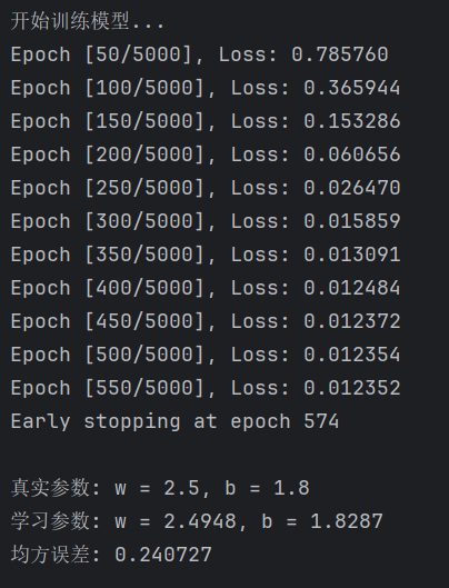
        print(f'\n真实参数: w = {true_w}, b = {true_b}')
        print(f'学习参数: w = {learned_w:.4f}, b = {learned_b:.4f}')
        print(f'均方误差: {mse:.6f}')

    return predictions


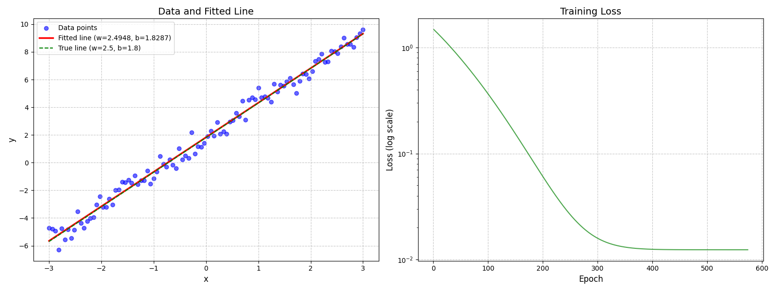
# 6. 可视化结果
def visualize_results(x, y, predictions, losses, true_w, true_b, learned_w, learned_b):
    # 创建两个图像
    fig, (ax1, ax2) = plt.subplots(1, 2, figsize=(16, 6))

    # 绘制数据点和拟合直线
    ax1.scatter(x.numpy(), y.numpy(), color='blue', alpha=0.6, label='Data points')
    ax1.plot(x.numpy(), predictions.numpy(), color='red', linewidth=2.5,
             label=f'Fitted line (w={learned_w:.4f}, b={learned_b:.4f})')
    ax1.plot(x.numpy(), true_w * x.numpy() + true_b, 'g--', linewidth=1.5, label=f'True line (w={true_w}, b={true_b})')
    ax1.set_xlabel('x', fontsize=12)
    ax1.set_ylabel('y', fontsize=12)
    ax1.set_title('Data and Fitted Line', fontsize=14)
    ax1.legend(fontsize=10)
    ax1.grid(True, linestyle='--', alpha=0.7)

    # 绘制损失曲线（对数尺度）
    ax2.semilogy(range(1, len(losses) + 1), losses, color='green', alpha=0.7)
    ax2.set_xlabel('Epoch', fontsize=12)
    ax2.set_ylabel('Loss (log scale)', fontsize=12)
    ax2.set_title('Training Loss', fontsize=14)
    ax2.grid(True, linestyle='--', alpha=0.7)

    plt.tight_layout()
    plt.show()


# 主函数
def main():
    # 生成数据（增加噪声水平以模拟更具挑战性的情况）
    x, y, true_w, true_b = generate_data(n_samples=100, noise_level=0.5)

    # 数据标准化
    x_stdized, y_stdized, x_mean, x_std, y_mean, y_std = standardize_data(x, y)

    # 初始化模型
    model = LinearRegression()

    # 训练模型（增加epochs，使用早停，调整学习率）
    print("开始训练模型...")
    losses = train_model(
        model, x_stdized, y_stdized,
        learning_rate=0.005,
        epochs=5000,
        patience=50,
        min_delta=1e-6
    )

    # 评估模型
    predictions = evaluate_model(model, x_stdized, y_stdized, true_w, true_b, x_mean, x_std, y_mean, y_std)

    # 获取学习到的参数用于可视化
    w_std = model.linear.weight.item()
    b_std = model.linear.bias.item()
    learned_w = w_std * (y_std / x_std)
    learned_b = b_std * y_std + y_mean - w_std * (y_std / x_std) * x_mean

    # 可视化结果
    visualize_results(x, y, predictions, losses, true_w, true_b, learned_w, learned_b)


if __name__ == "__main__":
    main()