


目录
一、基础知识
1.1 计算机视觉
视觉应用:
计算机视觉是一个飞速发展的一个领域,这多亏了深度学习。深度学习与计算机视觉可以帮助汽车,查明周围的行人和汽车,并帮助汽车避开 它们。还使得人脸识别技术变得更加效率和精准,你们即将能够体验到或早已体验过仅仅通过刷脸就能解锁手机或者门锁。当你解锁了手机,我猜手机上一定有很多分享图片的应用。 在上面,你能看到美食,酒店或美丽风景的图片。有些公司在这些应用上使用了深度学习技 术来向你展示最为生动美丽以及与你最为相关的图片。机器学习甚至还催生了新的艺术类型。
案例:图片识别、目标检测、图片风格迁移
1)你应该早就听说过图片分类,或者说图片识别。比如给出这张 64×64 的图片,让计算机去分辨出这是一只猫。

2)在计算机视觉中有个问题叫做目标检测,比如在一个无人驾驶项目中, 你不一定非得识别出图片中的物体是车辆,但你需要计算出其他车辆的位置,以确保自己能 够避开它们。所以在目标检测项目中,首先需要计算出图中有哪些物体,比如汽车,还有图 片中的其他东西,再将它们模拟成一个个盒子,或用一些其他的技术识别出它们在图片中的 位置。注意在这个例子中,在一张图片中同时有多个车辆,每辆车相对与你来说都有一个确切的距离。

3)神经网络实现的图片风格迁移,比如说你有一张图片,但 你想将这张图片转换为另外一种风格。所以图片风格迁移,就是你有一张满意的图片和一张 风格图片,实际上右边这幅画是毕加索的画作,而你可以利用神经网络将它们融合到一起, 描绘出一张新的图片。它的整体轮廓来自于左边,却是右边的风格,最后生成下面这张图片。 这种神奇的算法创造出了新的艺术风格,所以在这门课程中,你也能通过学习做到这样的事情。
计算机视觉应用面临的挑战:
数据的输入可能会非常大。举个例子,在过去的课程中,你们一般操作的都是 64×64 的小图片,实际上,它的数据量是 64×64×3,因为每张图片都有 3 个颜色通道。如果计算一下的话,可得知数据量为 12288(特征数目),所以我们的特征向量𝑥维度为 12288。这其实还好,因为 64×64 真的是很小的一张图片。
如果你要操作更大的图片,比如一张 1000×1000 的图片,它足有 1 兆那么大,但是特征 向量的维度达到了 1000×1000×3,因为有 3 个 RGB 通道,所以数字将会是 300 万
如果你要输入 300 万的数据量,这就意味着,特征向量𝑥的维度高达 300 万。所以在第 一隐藏层中,你也许会有 1000 个隐藏单元,而所有的权值组成了矩阵 𝑊[1]。如果你使用了标准的全连接网络,就像我们在第一门和第二门的课程里说的,这个矩阵的大小将会是 1000×300 万。因为现在𝑥的维度为3𝑚,3𝑚通常用来表示 300 万。这意味着矩阵𝑊[1]会有 30 亿个参数,这是个非常巨大的数字。在参数如此大量的情况下,难以获得足够的数据来防止神经网络发生过拟合和竞争需求,要处理包含 30 亿参数的神经网络,巨大的内存需求让人不太能接受。
解决措施:
但对于计算机视觉应用来说,你肯定不想它只处理小图片,你希望它同时也要能处理大图。为此,你需要进行卷积计算,它是卷积神经网络中非常重要的一块。
1.2 边缘检测示例
卷积运算是卷积神经网络最基本的组成部分,使用边缘检测作为入门样例。接下来,你会看到卷积是如何进行运算的。
检测的顺序:
我说过神经网络的前几层是如何检测边缘的,然后,后面的层有可能检测到物体的部分区域,更靠后的一些层可能检测到完整的物体,这个例子中就是人脸。接下来,你会看到如何在一张图片中进行边缘检测。
利用边缘监测算法我们可以检测出图片的横边和竖边。
过滤器认识:
看一个例子,这是一个 6×6 的灰度图像。因为是灰度图像,所以它是 6×6×1 的矩阵,而 不是 6×6×3 的,因为没有 RGB 三通道。为了检测图像中的垂直边缘,你可以构造一个 3×3 矩阵。在共用习惯中,在卷积神经网络的术语中,它被称为过滤器。我要构造一个 3×3 的过滤器,像这样 在论文它有时候会被称为核,而不是过滤器,但在这里,我将使用过滤器这个术语。对这个 6×6 的图像进行卷积运算,卷积运算用“∗”来表示,用 3×3 的过滤器对其进行卷积。
符号解释:
关于符号表示,有一些问题,在数学中“∗”就是卷积的标准标志,但是在 Python 中,这 个标识常常被用来表示乘法或者元素乘法。所以这个“∗”有多层含义,它是一个重载符号, 在这里,当“∗”表示卷积的时候我会特别说明。

卷积计算过程:
这个卷积运算的输出将会是一个 4×4 的矩阵,你可以将它看成一个 4×4 的图像。
为了计算第一个元素,在 4×4 左上角的那个元素,使 用 3×3 的过滤器,将其覆盖在输入图像,如下图所示。然后进行元素乘法运算。
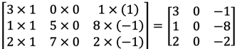
然后将该矩阵每个元素相加得到最左上角的元素,即3 + 1 + 2 + 0 + 0 + 0 + (−1) + (−8) + (−2) = −5
把这 9 个数加起来得到-5,当然,你可以把这 9 个数按任何顺序相加,我只是先写了第 一列,然后第二列,第三列。
接下来,为了弄明白第二个元素是什么,你要把蓝色的方块,向右移动一步,像这样, 把这些绿色的标记去掉:

继续做同样的元素乘法,然后加起来,所以是 0×1+5×1+7×1+1×0+8×0+ 2 × 0 + 2 × (−1) + 9 × (−1) + 5 × (−1) = −4。

接下来也是一样,继续右移一步,把 9 个数的点积加起来得到 0。
继续移得到 8,验证一下:2×1+9×1+5×1+7×0+3×0+1×0+4×(−1)+ 1 × (−1) + 3 × (−1) = 8。

接下来为了得到下一行的元素,现在把蓝色块下移,现在蓝色块在这个位置:

重复进行元素乘法,然后加起来。通过这样做得到-10。再将其右移得到-2,接着是 2, 3。以此类推,这样计算完矩阵中的其他元素。

为了说得更清楚一点,这个-16 是通过底部右下角的 3×3 区域得到的。
垂直边缘检测器:
因此 6×6 矩阵和 3×3 矩阵进行卷积运算得到 4×4 矩阵。这些图片和过滤器是不同维度的矩阵,但左边矩阵容易被理解为一张图片,中间的这个被理解为过滤器,右边的图片我们可以理解为另一张图片。这个就是垂直边缘检测器,
不同编程框架卷积运算函数
在 tensorflow 下,这个函数叫 tf.conv2d。在 Keras 这个框架,在这个框架下用 Conv2D 实现卷积运算。所有的编程框架都有一些函数来实现卷积运算。
为什么这个可以做垂直边缘检测呢?
示例:

这是一个简单的 6×6 图像,左边的一半是 10,右边一般是 0。如果你把它当 成一个图片,左边那部分看起来是白色的,像素值 10 是比较亮的像素值,右边像素值比较 暗,我使用灰色来表示 0,尽管它也可以被画成黑的。图片里,有一个特别明显的垂直边缘在图像中间,这条垂直线是从黑到白的过渡线,或者从白色到深色

所以,当你用一个 3×3 过滤器进行卷积运算的时候,这个 3×3 的过滤器可视化为下面这个样子,在左边有明亮的像素,然后有一个过渡,0 在中间,然后右边是深色的。卷积运算后,你得到的是右边的矩阵。如果你愿意,可以通过数学运算去验证。举例来说,最左上角的元素 0,就是由这个 3×3 块(绿色方框标记)经过元素乘积运算再求和得到的,10 × 1 + 10 × 1 + 10 × 1 + 10 × 0 + 10 × 0 + 10 × 0 + 10 × (−1) + 10 × (−1) + 10 × (−1) = 0。相反这个 30 是由这个(红色方框标记)得到的10×1+10×1+10×1+10×0+10×0+10×0+0×(−1)+0×(−1)+0× (−1) = 30。

如果把最右边的矩阵当成图像,它是这个样子。在中间有段亮一点的区域,对应检查到 这个 6×6 图像中间的垂直边缘。这里的维数似乎有点不正确,检测到的边缘太粗了。因为在 这个例子中,图片太小了。如果你用一个 1000×1000 的图像,而不是 6×6 的图片,你会发现其会很好地检测出图像中的垂直边缘。
在这个例子中,在输出图像中间的亮处,表示在图像中间有一个特别明显的垂直边缘。
从垂直边缘检测中可以得到的启发是,因为我们使用 3×3 的矩阵(过滤器),所以垂直边缘是一个 3×3 的区域,左边是明亮的像素,中间的并不需要 考虑,右边是深色像素。在这个 6×6 图像的中间部分,明亮的像素在左边,深色的像素在右 边,就被视为一个垂直边缘,卷积运算提供了一个方便的方法来发现图像中的垂直边缘。
1.3 更多边缘检测内容
图片边缘有两种渐变方式,一种是由明变暗,另一种是由暗变明。以垂直边缘检测为例,下图展示了两种方式的区别。实际应用中,这两种渐变方式并不影响边缘检测结果,可以对输出图片取绝对值操作,得到同样的结果。

垂直边缘检测和水平边缘检测的滤波器算子如下所示:

下图展示一个水平边缘检测的例子:

除了上面提到的这种简单的Vertical、Horizontal滤波器之外,还有其它常用的filters,例如Sobel filter和Scharr filter。这两种滤波器的特点是增加图片中心区域的权重。

上图展示的是垂直边缘检测算子,水平边缘检测算子只需将上图顺时针翻转90度即可。
在深度学习中,如果我们想检测图片的各种边缘特征,而不仅限于垂直边缘和水平边缘,那么filter的数值一般需要通过模型训练得到,类似于标准神经网络中的权重W一样由梯度下降算法反复迭代求得。CNN的主要目的就是计算出这些filter的数值。确定得到了这些filter后,CNN浅层网络也就实现了对图片所有边缘特征的检测。
1.4 Padding
按照我们上面讲的图片卷积,如果原始图片尺寸为n x n,filter尺寸为f x f,则卷积后的图片尺寸为(n-f+1) x (n-f+1),注意f一般为奇数。这样会带来两个问题:
-
卷积运算后,输出图片尺寸缩小
-
原始图片边缘信息对输出贡献得少,输出图片丢失边缘信息
为了解决图片缩小的问题,可以使用padding方法,即把原始图片尺寸进行扩展,扩展区域补零,用p来表示每个方向扩展的宽度。

经过padding之后,原始图片尺寸为(n+2p) x (n+2p),filter尺寸为f x f,则卷积后的图片尺寸为(n+2p-f+1) x (n+2p-f+1)。若要保证卷积前后图片尺寸不变,则p应满足:

没有padding操作 ![]() ,我们称之为“Valid convolutions”(图片变小);有padding操作,
,我们称之为“Valid convolutions”(图片变小);有padding操作,![]() 我们称之为“Same convolutions”(图片不变)。
我们称之为“Same convolutions”(图片不变)。
f为奇数的原因:
1)达到对称填充
2)只有一个中心点
1.5 卷积步长
Stride表示filter在原图片中水平方向和垂直方向每次的步进长度。之前我们默认stride=1。若stride=2,则表示filter每次步进长度为2,即隔一点移动一次。

我们用s表示stride长度,p表示padding长度,如果原始图片尺寸为n x n,filter尺寸为f x f,则卷积后的图片尺寸为:

上式中,⌊⋯⌋表示向下取整。
值得一提的是,相关系数(cross-correlations)与卷积(convolutions)之间是有区别的。实际上,真正的卷积运算会先将filter绕其中心旋转180度,然后再将旋转后的filter在原始图片上进行滑动计算。filter旋转如下所示:
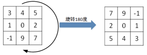
比较而言,相关系数的计算过程则不会对filter进行旋转,而是直接在原始图片上进行滑动计算。
其实,目前为止我们介绍的CNN卷积实际上计算的是相关系数,而不是数学意义上的卷积。但是,为了简化计算,我们一般把CNN中的这种“相关系数”就称作卷积运算。之所以可以这么等效,是因为滤波器算子一般是水平或垂直对称的,180度旋转影响不大;而且最终滤波器算子需要通过CNN网络梯度下降算法计算得到,旋转部分可以看作是包含在CNN模型算法中。总的来说,忽略旋转运算可以大大提高CNN网络运算速度,而且不影响模型性能。
1.6 三维卷积
我们了解了卷积的操作,那么如何处理图片的RGB数据呢?就是使用三维卷积,也就是可以理解成进行三次卷积操作
对于3通道的RGB图片,其对应的滤波器算子同样也是3通道的。例如一个图片是6 x 6 x 3,分别表示图片的高度(height)、宽度(weight)和通道(#channel)。
3通道图片的卷积运算与单通道图片的卷积运算基本一致。过程是将每个单通道(R,G,B)与对应的filter进行卷积运算求和,然后再将3通道的和相加,得到输出图片的一个像素值。

不同通道的滤波算子可以不相同。例如R通道filter实现垂直边缘检测,G和B通道不进行边缘检测,全部置零,或者将R,G,B三通道filter全部设置为水平边缘检测。
为了进行多个卷积运算,实现更多边缘检测,可以增加更多的滤波器组。例如设置第一个滤波器组实现垂直边缘检测,第二个滤波器组实现水平边缘检测。这样,不同滤波器组卷积得到不同的输出,个数由滤波器组决定。

![]()
总结:
这个对立方体卷积的概念真的很有用,你现在可以用它的一小部分直接在三个通道的 RGB 图像上进行操作。更重要的是,你可以检测两个特征,比如垂直和水平边缘或者 10 个 或者 128 个或者几百个不同的特征,并且输出的通道数会等于你要检测的特征数。
1.7 单层卷积网络
卷积神经网络的单层结构如下所示:

相比之前的卷积过程,CNN的单层结构多了激活函数ReLU和偏移量b。整个过程与标准的神经网络单层结构非常类似:

卷积运算对应着上式中的乘积运算,滤波器组数值对应着权重 W[l],所选的激活函数为ReLU。
我们来计算一下上图中参数的数目:每个滤波器组有3x3x3=27个参数,还有1个偏移量b,则每个滤波器组有27+1=28个参数,两个滤波器组总共包含28x2=56个参数。我们发现,选定滤波器组后,参数数目与输入图片尺寸无关。所以,就不存在由于图片尺寸过大,造成参数过多的情况。例如一张1000x1000x3的图片,标准神经网络输入层的维度将达到3百万,而在CNN中,参数数目只由滤波器组决定,数目相对来说要少得多,这是CNN的优势之一。
最后,我们总结一下描述卷积神经网络中的一层,以𝑙层为例。也就是卷积层的各种标记。

其中:

1.8 简单卷积网络示例
下面介绍一个简单的CNN网络模型:
示例:通过卷积神经网络图片分类或图片识别
图片输入定义为𝑥,大小39×39×3,最终输出结果用 0 或 1 表示,这是一个分类问题。
1)![]() 即高度和宽度都等于 39
即高度和宽度都等于 39![]()
即 0 层的通道数为3。
2)第一层我们用一个 3×3 的过滤器来提取特征(每个过滤器组维度 3×3×3),那么𝑓[1] = 3,因为过滤器时 3×3 的矩阵。𝑠[1] = 1,𝑝[1] = 0,所以高度和宽度使用 same 卷积。如果有 10 个过滤器,神经网络下一层的激活值为 37×37×10,37 是公式
![]() 计算结果,它是一个 vaild 卷积,这是输出结果的大小。
计算结果,它是一个 vaild 卷积,这是输出结果的大小。
第一层标记为![]()
![]() 等于第一层中过滤器的个数,这(37×37×10)是第一层激活值的维度。
等于第一层中过滤器的个数,这(37×37×10)是第一层激活值的维度。
3)第二层我们采用的过滤器是 5×5 的矩阵(每个过滤器组维度 5×5×10)
在标记法中,神经网络下一层的𝑓 = 5,即𝑓[2] = 5步幅为 2,即𝑠[2] = 2。padding 为 0,即𝑝[2] = 0,且有 20 个过滤器。
输出结果会是一张新图像,这次的输出结果为 17×17×20,因为步幅是 2,维度缩小得很快,大小从 37×37 减小到 17×17,减小了一半还多,过滤器是 20 个,所以通道数也是 20,17×17×20 即激活值𝑎[2]的维度。因此![]()
4)最后一个卷积层,假设过滤器还是 5×5,步幅为 2,即𝑓[2] = 5,𝑠[3] = 2,计算过程我跳过了,最后输出为 7×7×40,假设使用 了 40 个过滤器。padding 为 0,40 个过滤器,最后结果为 7×7×40。
上述总结:
到此,这张 39×39×3 的输入图像就处理完毕了,为图片提取了 7×7×40 个特征,计算出 来就是 1960 个特征。然后对该卷积进行处理,可以将其平滑或展开成 1960 个单元。平滑处理后可以输出一个向量,其填充内容是 logistic 回归单元还是 softmax 回归单元,完全取决于我们是想识图片上有没有猫,还是想识别𝐾种不同对象中的一种,用𝑦表示最终神经网络 的预测输出。
值得一提的是,随着CNN层数增加,![]() 一般逐渐减小,而
一般逐渐减小,而 ![]()
一般逐渐增大。
总结:
CNN有三种类型的layer:
-
Convolution层(CONV)
-
Pooling层(POOL)
-
Fully connected层(FC)
一个典型的卷积神经网络通常有三层,一个是卷积层,我们常常用 Conv 来标注上一 个例子,我用的就是 CONV。
还有两种常见类型的层,我们后面讲。一个是池化层, 我们称之为 POOL。最后一个是全连接层,用 FC 表示。
虽然仅用卷积层也有可能构建出很好的神经网络,但大部分神经网络架构师依然会添加池化层和全连接层。幸运的是,池化层和全连接层比卷积层更容易设计。
1.9 池化层
Pooling layers是CNN中用来减小尺寸,提高运算速度的,同样能减小noise影响,让各特征更具有健壮性。
Pooling layers的做法比convolution layers简单许多,没有卷积运算,仅仅是在滤波器算子滑动区域内取最大值,即max pooling,这是最常用的做法。注意,超参数p很少在pooling layers中使用。
Max pooling的好处是只保留区域内的最大值(特征),忽略其它值,降低noise影响,提高模型健壮性。而且,max pooling需要的超参数仅为滤波器尺寸f和滤波器步进长度s,没有其他参数需要模型训练得到,计算量很小。
如果是多个通道,那么就每个通道单独进行max pooling操作。
除了max pooling之外,还有一种做法:average pooling。顾名思义,average pooling就是在滤波器算子滑动区域计算平均值。
实际应用中,max pooling比average pooling更为常用。
1.10 卷积神经网络示例
下面介绍一个简单的数字识别的CNN例子:
图中,CON层后面紧接一个POOL层,CONV1和POOL1构成第一层,CONV2和POOL2构成第二层。特别注意的是FC3和FC4为全连接层FC,它跟标准的神经网络结构一致。最后的输出层(softmax)由10个神经元构成。
参数选择:
此例中的卷积神经网络很典型,看上去它有很多超参数,关于如何选定这些参数,后面我提供更多建议。常规做法是,尽量不要自己设置超参数,而是查看文献中别人采用了哪些超参数,选一个在别人任务中效果很好的架构,那么它也有可能适用于你自己的应用程序。
现在,我想指出的是,随着神经网络深度的加深,高度𝑛𝐻 和宽度𝑛𝑊 通常都会减少,前面我就提到过,从 32×32 到 28×28,到 14×14,到 10×10,再到 5×5。所以随着层数增加,高度和宽度都会减小,而通道数量会增加,从 3 到 6 到 16 不断增加,然后得到一个全连接层。
在神经网络中,另一种常见模式就是一个或多个卷积后面跟随一个池化层,然后一个或多个卷积层后面再跟一个池化层,然后是几个全连接层,最后是一个 softmax。这是神经网络的另一种常见模式。
神经网络的激活值形状,激活值大小和参数数量

几点要注意,第一,池化层和最大池化层没有参数;第二卷积层的参数相对较少,前面课上我们提到过,其实许多参数都存在于神经网络的全连接层。观察可发现,随着神经网络的加深,激活值尺寸会逐渐变小,如果激活值尺寸下降太快,也会影响神经网络性能。示 例中,激活值尺寸在第一层为 6000,然后减少到 1600,慢慢减少到 84,最后输出 softmax 结果。我们发现,许多卷积网络都具有这些属性,模式上也相似。
总结:
一个卷积神经网络包括卷积层、池化层和全 连接层。许多计算机视觉研究正在探索如何把这些基本模块整合起来,构建高效的神经网络, 整合这些基本模块确实需要深入的理解。根据我的经验,找到整合基本构造模块最好方法就 是大量阅读别人的案例。
1.11 为什么使用卷积
相比标准神经网络,CNN的优势之一就是参数数目要少得多。参数数目少的原因有两个:
-
参数共享:一个特征检测器(例如垂直边缘检测)对图片某块区域有用,同时也可能作用在图片其它区域。
-
连接的稀疏性:因为滤波器算子尺寸限制,每一层的每个输出只与输入部分区域内有关。
除此之外,由于CNN参数数目较小,所需的训练样本就相对较少,从而一定程度上不容易发生过拟合现象。而且,CNN比较擅长捕捉区域位置偏移。也就是说CNN进行物体检测时,不太受物体所处图片位置的影响,增加检测的准确性和系统的健壮性。
二、测验
1. 你认为把下面这个过滤器应用到灰度图像会怎么样?
- 会检测45度边缘
- 会检测垂直边缘
- 会检测水平边缘
- 会检测图像对比度
2
2. 假设你的输入是一个300×300的彩色(RGB)图像,而你没有使用卷积神经网络。 如果第一个隐藏层有100个神经元,每个神经元与输入层进行全连接,那么这个隐藏层有多少个参数(包括偏置参数)?
27,000,100 (300*300*3*100+100(偏置))
3. 假设你的输入是300×300彩色(RGB)图像,并且你使用卷积层和100个过滤器,每个过滤器都是5×5的大小,请问这个隐藏层有多少个参数(包括偏置参数)?
7600( (5*5*3+1)*100 )
4. 你有一个63x63x16的输入,并使用大小为7×7的32个过滤器进行卷积,使用步幅为2和无填充,请问输出是多少?
29*29*32 【(( 63+2*0-7 )/2)+1】0是padding
5. 你有一个15x15x8的输入,并使用“pad = 2”进行填充,填充后的尺寸是多少?
19*19*8
6. 你有一个63x63x16的输入,有32个过滤器进行卷积,每个过滤器的大小为7×7,步幅为1,你想要使用“same”的卷积方式,请问pad的值是多少?
3【(7-1)/2】
7. 你有一个32x32x16的输入,并使用步幅为2、过滤器大小为2的最大化池,请问输出是多少?
16*16*16
8. 因为池化层不具有参数,所以它们不影响反向传播的计算。
错误。
9. 在视频中,我们谈到了“参数共享”是使用卷积网络的好处。关于参数共享的下列哪个陈述是正确的?(检查所有选项。)
- 它减少了参数的总数,从而减少过拟合。
- 它允许在整个输入值的多个位置使用特征检测器。
- 它允许为一项任务学习的参数即使对于不同的任务也可以共享(迁移学习)。
- 它允许梯度下降将许多参数设置为零,从而使得连接稀疏。
2,4。
10. 在课堂上,我们讨论了“稀疏连接”是使用卷积层的好处。这是什么意思?
- 正则化导致梯度下降将许多参数设置为零。
- 每个过滤器都连接到上一层的每个通道。
- 下一层中的每个激活只依赖于前一层的少量激活。
- 卷积网络中的每一层只连接到另外两层。
3。
三、编程作业
3.1 一步步实现卷积神经网络
下面将用 numpy实现卷积(CONV)和池化(POOL)层,包括正向传播和向后传播。
符号:
上标[𝑙] 表示第 𝑙𝑡ℎ层对象,例如:𝑎[4] 是 第四层激活,𝑊[5] 和 𝑏[5]是第五层参数。
上标 (i)表示第 i个示例,例如:𝑥(𝑖)是第 i个训练样本输入。
3.1.1 导包
numpy是使用Python进行科学计算的基本软件包。
matplotlib是一个用于在Python中绘制图形的库。
np.random.seed(1)用于使所有随机函数调用保持一致。
3.1.2 作业大纲
您将实现卷积神经网络的构建模块!
- Convolution functions, including:
- Zero Padding
- Convolve window
- Convolution forward
- Convolution backward (optional)
- Pooling functions, including:
- Pooling forward
- Create mask
- Distribute value
- Pooling backward (optional)
这里需要您从头开始在numpy中实现这些功能。 在下一个目录中,您将使用这些函数的TensorFlow等效项来构建以下模型。

注意,对于每个正向功能,都有其对应的向后等效项。 因此,在正向传播中的每一步中,您都需要将一些参数存储在缓存中。 这些参数用于在反向传播期间计算梯度。
3.1.3 卷积神经网络
尽管编程框架使卷积易于使用,但它们仍然是深度学习中最难理解的概念之一。 卷积层将输入体积转换为不同大小的输出体积,如下所示。

在这一部分,您将构建卷积层的每个步骤。 您将首先实现两个辅助函数:
一个用于零填充,
另一个用于计算卷积函数本身。
3.1.4 零填充
零填充会在图像的边界周围添加零:

填充的主要好处如下:
- 它使您可以使用CONV层而不必缩小卷的高度和宽度。 这对于构建更深的网络很重要,因为否则高度/宽度会随着您进入更深的层而缩小。 一个重要的特殊情况是“相同”卷积,其中高度/宽度在下一层之后被精确保留。
- 它可以帮助我们将更多信息保留在图像的边缘。 如果不进行填充,则下一层的值很少会受到像素作为图像边缘的影响。
我们使用numpy提供的pad参数来进行padding操作,需要传的几个参数分别是array,然后就是三个维度上分别扩展多少位(arr3D为一个三维数组,我们不希望变成4维所以第一个均为0,然后第二维第三维上下左右分别加上几个0),然后constant表示填充(默认填充0)。
import numpy as np

# 填充
arr3D = np.array([[[1, 1, 2, 2, 3, 4],
                   [1, 1, 2, 2, 3, 4],
                   [1, 1, 2, 2, 3, 4]],

                  [[0, 1, 2, 3, 4, 5],
                   [0, 1, 2, 3, 4, 5],
                   [0, 1, 2, 3, 4, 5]],

                  [[1, 1, 2, 2, 3, 4],
                   [1, 1, 2, 2, 3, 4],
                   [1, 1, 2, 2, 3, 4]]])

print('constant:  \n' + str(np.pad(arr3D, ((0, 0), (1, 1), (2, 2)), 'constant')))


#输出结果

[[[0 0 0 0 0 0 0 0 0 0]
  [0 0 1 1 2 2 3 4 0 0]
  [0 0 1 1 2 2 3 4 0 0]
  [0 0 1 1 2 2 3 4 0 0]
  [0 0 0 0 0 0 0 0 0 0]]

 [[0 0 0 0 0 0 0 0 0 0]
  [0 0 0 1 2 3 4 5 0 0]
  [0 0 0 1 2 3 4 5 0 0]
  [0 0 0 1 2 3 4 5 0 0]
  [0 0 0 0 0 0 0 0 0 0]]

 [[0 0 0 0 0 0 0 0 0 0]
  [0 0 1 1 2 2 3 4 0 0]
  [0 0 1 1 2 2 3 4 0 0]
  [0 0 1 1 2 2 3 4 0 0]
  [0 0 0 0 0 0 0 0 0 0]]]
修改 print('constant: \n' + str(np.pad(arr3D, ((1, 1), (1, 1), (2, 2)), 'constant')))
输出结果:
[[[0 0 0 0 0 0 0 0 0 0]
  [0 0 0 0 0 0 0 0 0 0]
  [0 0 0 0 0 0 0 0 0 0]
  [0 0 0 0 0 0 0 0 0 0]
  [0 0 0 0 0 0 0 0 0 0]]

 [[0 0 0 0 0 0 0 0 0 0]
  [0 0 1 1 2 2 3 4 0 0]
  [0 0 1 1 2 2 3 4 0 0]
  [0 0 1 1 2 2 3 4 0 0]
  [0 0 0 0 0 0 0 0 0 0]]

 [[0 0 0 0 0 0 0 0 0 0]
  [0 0 0 1 2 3 4 5 0 0]
  [0 0 0 1 2 3 4 5 0 0]
  [0 0 0 1 2 3 4 5 0 0]
  [0 0 0 0 0 0 0 0 0 0]]

 [[0 0 0 0 0 0 0 0 0 0]
  [0 0 1 1 2 2 3 4 0 0]
  [0 0 1 1 2 2 3 4 0 0]
  [0 0 1 1 2 2 3 4 0 0]
  [0 0 0 0 0 0 0 0 0 0]]

 [[0 0 0 0 0 0 0 0 0 0]
  [0 0 0 0 0 0 0 0 0 0]
  [0 0 0 0 0 0 0 0 0 0]
  [0 0 0 0 0 0 0 0 0 0]
[0 0 0 0 0 0 0 0 0 0]]]具体解释参考博客:深度学习-np.pad 填充详解_小飞猪666的博客-CSDN博客
我们试着可视化一下:
import numpy as np
import h5py
import matplotlib.pyplot as plt

# 张量填充
def zero_pad(X, pad):
    """
    Pad with zeros all images of the dataset X. The padding is applied to the height and width of an image,
    as illustrated in Figure 1.
    Argument:
    X -- python numpy array of shape (m,  n_C, n_H, n_W) representing a batch of m images
    pad -- integer, amount of padding around each image on vertical and horizontal dimensions
    Returns:
    X_pad -- padded image of shape (m, n_C, n_H + 2*pad, n_W + 2*pad)
    """
    X_pad = np.pad(X, ((0, 0), (0, 0), (pad, pad), (pad, pad)), 'constant', constant_values=0)
    return X_pad

if __name__ == '__main__':
    # 1.1 生成一个四维数组(图像基本上都是4D张量)
    np.random.seed(1)
    # (samples,channels,height,width)
    x = np.random.randn(4, 2, 3, 3)
    x_paded = zero_pad(x, 2)
    print('x: \n' + str(x))
    print('x_paded: \n' + str(x_paded))

    # # 绘制图
    fig, axarr = plt.subplots(1, 2)  # 绘制一行两列画布
    axarr[0].set_title('x')  # 第一列的画布设置title
    axarr[0].imshow(x[0, 0, :, :])  # 将第一个样本的第一个channel的矩阵可视化 3 X 2
    axarr[1].set_title('x_paded')
    axarr[1].imshow(x_paded[0, 0, :, :])
    plt.show()
输出结果:

3.1.5 卷积的第一步
在这一部分中,实现卷积的单个步骤,其中将过滤器应用于输入的单个位置。 这将用于构建卷积单元,该卷积单元:
- Takes an input volume
- Applies a filter at every position of the input
- Outputs another volume (usually of different size)

在计算机视觉应用程序中,左侧矩阵中的每个值都对应一个像素值,我们应用3x3 过滤器将元素的值与原始矩阵相乘,然后将它们相加进行卷积。 在练习的第一步中,您将实现卷积的单个步骤,相当于仅对一个位置应用过滤器以获得单个实值输出。
在本笔记本的后面,您将将此功能应用于输入的多个位置以实现完整的卷积运算。
练习:实现conv_single_step()
def conv_single_step(a_slice_prev, W, b):
    # https://blog.csdn.net/zenghaitao0128/article/details/78715140
    """
    Apply one filter defined by parameters W on a single slice (a_slice_prev) of the output activation
    of the previous layer.
    Arguments:
    a_slice_prev -- slice of input data of shape (n_C_prev, f, f)
    W -- Weight parameters contained in a window - matrix of shape (n_C_prev, f, f)
    b -- Bias parameters contained in a window - matrix of shape (1, 1, 1)
    Returns:
    Z -- a scalar value, result of convolving the sliding window (W, b) on a slice x of the input data
    """
    s = np.multiply(a_slice_prev, W) + b
    Z = np.sum(s)
    return Z

if __name__ == '__main__':

    # 1.2 卷积的第一步
    np.random.seed(1)
    a_slice_prev = np.random.randn(3, 4, 4)
    W = np.random.randn(3, 4, 4)
    b = np.random.randn(1, 1, 1)
    Z = conv_single_step(a_slice_prev, W, b)
    print('a_slice_prev:\n' + str(a_slice_prev))
    print('W:\n' + str(W))
    print('b:\n' + str(b))
    print("Z =", Z)
输出结果:
Z = -23.160212202520783.1.6 卷积神经网络-前向传播
在前向传递中,您将使用许多过滤器并将它们卷积在输入上。 每个“卷积”都会为您提供2D矩阵输出。 然后,您将堆叠这些输出以获得3D输出:

计算卷积后图片大小公式如下:
import numpy as np
import h5py
import matplotlib.pyplot as plt

# 张量填充
def zero_pad(X, pad):
    """
    Pad with zeros all images of the dataset X. The padding is applied to the height and width of an image,
    as illustrated in Figure 1.
    Argument:
    X -- python numpy array of shape (m,  n_C, n_H, n_W) representing a batch of m images
    pad -- integer, amount of padding around each image on vertical and horizontal dimensions
    Returns:
    X_pad -- padded image of shape (m, n_C, n_H + 2*pad, n_W + 2*pad)
    """
    X_pad = np.pad(X, ((0, 0), (0, 0), (pad, pad), (pad, pad)), 'constant', constant_values=0)
    return X_pad


# 卷积网络-前向传播
def conv_forward(A_prev, W, b, hparameters):
    """
    Implements the forward propagation for a convolution function
    Arguments:
    A_prev -- output activations of the previous layer, numpy array of shape (m, n_C_prev, n_H_prev, n_W_prev)
    W -- Weights, numpy array of shape (n_C, n_C_prev, f, f)
    b -- Biases, numpy array of shape (1, n_C,1, 1)
    hparameters -- python dictionary containing "stride" and "pad"
    Returns:
    Z -- conv output, numpy array of shape (m, n_C, n_H, n_W)
    cache -- cache of values needed for the conv_backward() function
    """

    # 第0层 样本数目:10 大小: 维度:3 矩阵:4 x 4
    # 输入维度 3 x 4 x 4
    (m, n_C_prev, n_H_prev, n_W_prev) = A_prev.shape

    # 第一层过滤器 每个过滤器组:维度:3  矩阵大小:2 x 2
    # 权重维度 8 x 3 x 2 x 2
    (n_C, n_C_prev, f, f) = W.shape

    # 步幅: 1 填充:2
    stride = hparameters['stride']
    pad = hparameters['pad']

    # 计算卷积计算后的输出 大小 7 x 7
    # 输出维度 8 x 7 x 7
    n_H = 1 + int((n_H_prev + 2 * pad - f) / stride)
    n_W = 1 + int((n_W_prev + 2 * pad - f) / stride)

    # 初始化输出 Z
    # 10 x 8 x 7 x 7
    Z = np.zeros((m, n_C, n_H, n_W))

    # 创建 A_prev_pad 通过用0填充 A_prev
    # 填充后 10 x 3 x 8 x 8
    A_prev_pad = zero_pad(A_prev, pad)  # 样本数目:10 大小:8x8 维度:3
    for i in range(m):  # 遍历训练样本
        a_prev_pad = A_prev_pad[i]  # 选择 ith 训练样本
        print(a_prev_pad)
        for h in range(n_H):  # n_H:7  在垂直轴上循环遍历
            for w in range(n_W):  # n_W:在水平轴上循环遍历
                for c in range(n_C):  # 遍历过滤器数目
                    # 寻找当前切片
                    vert_start = h * stride
                    vert_end = vert_start + f
                    horiz_start = w * stride
                    horiz_end = horiz_start + f
                    # 使用边角定义a_prev_pad的(3D)切片
                    a_slice_prev = a_prev_pad[:, vert_start:vert_end, horiz_start:horiz_end]
                    print(a_slice_prev)
                    # 用正确的滤波器W和偏差b对(3D)切片进行卷积,以返回一个输出神经元。
                    Z[i, c, h, w] = np.sum(np.multiply(a_slice_prev, W[c, :, :, :]) + b[:, c, :, :])
    # 确保输出 shape 是正确的
    assert (Z.shape == (m, n_C, n_H, n_W))

    # 保存信息到 "cache"中
    cache = (A_prev, W, b, hparameters)

    return Z, cache


if __name__ == '__main__':
    # 1.3 卷积神经网络-前向传播
    np.random.seed(1)
    # (sample,channels,height,width)
    # 样本数:10 维度:3 矩阵大小:4 x 4
    A_prev = np.random.randn(10, 3, 4, 4)
    # 过滤器数目:8  维度:3 大小 2x2
    W = np.random.randn(8, 3, 2, 2)
    # 偏置数目:1  维度:8 大小 1x1
    b = np.random.randn(1, 8, 1, 1)
    hparameters = {"pad": 2, "stride": 1}
    Z, cache_conv = conv_forward(A_prev, W, b, hparameters)
    print("Z's mean =", np.mean(Z))
    print("cache_conv[0][1][2][3] =", cache_conv[0][1][2][3])
输出结果:
Z's mean = 0.18479238427393258
cache_conv[0][1][2][3] = [-0.37528495 -0.63873041 0.42349435 0.07734007]
最后,CONV层还应包含一个激活,在这种情况下,我们将添加以下代码行:
# Convolve the window to get back one output neuron
Z[i, h, w, c] = ...
# Apply activation
A[i, h, w, c] = activation(Z[i, h, w, c])
3.1.7 池化层
池化层减少了输入的高度和宽度。 它有助于减少计算量,并有助于使特征检测器在输入中的位置更加不变。 池化层的两种类型是:
- 最大池层
- 平均池层

这些池化层没有用于反向传播训练的参数。 但是,它们具有超参数,例如窗口大小𝑓。 这指定了您要计算最大值或平均值的 fxf 窗口的高度和宽度。
3.1.8 前向池
现在,您将在同一方法中实现MAX-POOL和AVG-POOL。
练习:实现池化层的前向传递。 请遵循以下的提示。
提醒:由于没有填充,公式如下:

import numpy as np
import h5py
import matplotlib.pyplot as plt


# 前向池
def pool_forward(A_prev, hparameters, mode="max"):
    """
    Implements the forward pass of the pooling layer
    Arguments:
    A_prev -- Input data, numpy array of shape (m, n_C_prev, n_H_prev, n_W_prev)
    hparameters -- python dictionary containing "f" and "stride"
    mode -- the pooling mode you would like to use, defined as a string ("max" or "average")
    Returns:
    A -- output of the pool layer, a numpy array of shape (m, n_C, n_H, n_W)
    cache -- cache used in the backward pass of the pooling layer, contains the input and hparameters
    """

    # 输出层 2 x 3 x 4 x 4
    # 样本数目:2 大小 维度 3 4x4
    (m, n_C_prev, n_H_prev, n_W_prev) = A_prev.shape

    # filter 4  步长:1
    f = hparameters["f"]
    stride = hparameters["stride"]

    # 定义输出层维度  3 x 1 x 1
    n_H = int(1 + (n_H_prev - f) / stride)
    n_W = int(1 + (n_W_prev - f) / stride)
    n_C = n_C_prev

    # 初始化输出矩阵 A 2 x 3 x 1 x 1
    A = np.zeros((m, n_C, n_H, n_W))

    for i in range(m):  # 遍历训练样本 目前为2
        for h in range(n_H):  # 从垂直方向遍历
            for w in range(n_W):  # 从水平方向遍历
                for c in range(n_C):  # 循环通道数目

                    # Find the corners of the current "slice" (≈4 lines)
                    vert_start = h * stride
                    vert_end = vert_start + f
                    horiz_start = w * stride
                    horiz_end = horiz_start + f

                    # Use the corners to define the current slice on the ith training example of A_prev, channel c. (≈1 line)
                    a_prev_slice = A_prev[i, c, vert_start:vert_end, horiz_start:horiz_end]

                    # Compute the pooling operation on the slice. Use an if statment to differentiate the modes. Use np.max/np.mean.
                    if mode == "max":
                        A[i, c, h, w] = np.max(a_prev_slice)
                    elif mode == "average":
                        A[i, c, h, w] = np.mean(a_prev_slice)

            ### END CODE HERE ###

            # Store the input and hparameters in "cache" for pool_backward()
    cache = (A_prev, hparameters)

    # Making sure your output shape is correct
    assert (A.shape == (m, n_C, n_H, n_W))

    return A, cache

if __name__ == '__main__':
    np.random.seed(1)
    # 1.4 池化层-前向池
    A_prev = np.random.randn(2, 3, 4, 4)
    hparameters = {"stride": 1, "f": 4}

    A, cache = pool_forward(A_prev, hparameters)
    print("mode = max")
    print("A =", A)
    print()
    A, cache = pool_forward(A_prev, hparameters, mode="average")
    print("mode = average")
    print("A =", A)
输出结果:
mode = max
A = [[[[1.74643509]]
  [[1.47073986]]
  [[1.22515585]]]
 [[[1.07125243]]
  [[1.57546791]]
  [[1.34710546]]]]
mode = average
A = [[[[ 0.31894709]]
  [[-0.31345433]]
  [[ 0.04513805]]]
 [[[-0.17976856]]
  [[-0.05195481]]
  [[ 0.01859955]]]]
恭喜你! 现在,您已经实现了卷积网络所有层的前向传递。
3.1.9 卷积神经网络中的反向传播
在现代深度学习框架中,您只需要实现前向传递,该框架就可以处理后向传递,因此大多数深度学习工程师无需理会后向传递的细节。 卷积网络的后向传递很复杂。 但是,如果您愿意,可以在noteBook的此可选部分中进行操作,以了解卷积网络中反向传播。
在较早的课程中,当您实现了一个简单的(完全连接的)神经网络时,您就使用了反向传播来计算关于更新参数的成本的导数。 类似地,在卷积神经网络中,您可以计算成本的导数以更新参数。 反向传播方程并非无关紧要的,但在下面简要介绍了它们。
卷积层后向传播:
让我们从实现CONV层的向后传递开始。
计算dA:
这是关于某种过滤器的成本𝑊𝑐去计算dA的一种公式

在代码中,在适当的for循环内,此公式转换为
da_prev_pad[:, vert_start:vert_end, horiz_start:horiz_end] += W[c, :, :, :] * dZ[i, c, h, w]计算dW
在代码中,在适当的for循环内,此公式转换为:
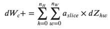
dW[c, :, :, :] += a_slice * dZ[i, c, h, w]计算db:

在代码中,在适当的for循环内,此公式转换为:
db[:, c, :, :] += dZ[i, c, h, w]练习:在下面实现conv_backward函数。 您应该总结所有训练示例,过滤器,高度和宽度。 然后,您应该使用上面的公式1、2和3计算导数。
import numpy as np
import h5py
import matplotlib.pyplot as plt


# 卷积层-后向传播
def conv_backward(dZ, cache):
    """
    实现卷积层的后向传播
    Arguments:
    dZ -- gradient of the cost with respect to the output of the conv layer (Z), numpy array of shape (m, n_C, n_H, n_W)
    cache -- cache of values needed for the conv_backward(), output of conv_forward()
    Returns:
    dA_prev -- gradient of the cost with respect to the input of the conv layer (A_prev),
               numpy array of shape (m, n_C_prev, n_H_prev, n_W_prev)
    dW -- gradient of the cost with respect to the weights of the conv layer (W)
          numpy array of shape (n_C, n_C_prev, f, f)
    db -- gradient of the cost with respect to the biases of the conv layer (b)
          numpy array of shape (1, n_C, 1, 1)
    """

    (A_prev, W, b, hparameters) = cache

    (m, n_C_prev, n_H_prev, n_W_prev) = A_prev.shape

    (n_C, n_C_prev, f, f) = W.shape

    stride = hparameters['stride']
    pad = hparameters['pad']

    # Retrieve dimensions from dZ's shape
    (m, n_C, n_H, n_W) = dZ.shape

    # Initialize dA_prev, dW, db with the correct shapes
    dA_prev = np.zeros((m, n_C_prev, n_H_prev, n_W_prev))
    dW = np.zeros((n_C, n_C_prev, f, f))
    db = np.zeros((1, n_C, 1, 1))

    # Pad A_prev and dA_prev
    A_prev_pad = zero_pad(A_prev, pad)
    dA_prev_pad = zero_pad(dA_prev, pad)

    for i in range(m):  # loop over the training examples

        # select ith training example from A_prev_pad and dA_prev_pad
        a_prev_pad = A_prev_pad[i]
        da_prev_pad = dA_prev_pad[i]

        for h in range(n_H):  # loop over vertical axis of the output volume
            for w in range(n_W):  # loop over horizontal axis of the output volume
                for c in range(n_C):  # loop over the channels of the output volume

                    # Find the corners of the current "slice"
                    vert_start = h * stride
                    vert_end = vert_start + f
                    horiz_start = w * stride
                    horiz_end = horiz_start + f

                    # Use the corners to define the slice from a_prev_pad
                    a_slice = a_prev_pad[:, vert_start:vert_end, horiz_start:horiz_end]

                    # Update gradients for the window and the filter's parameters using the code formulas given above
                    da_prev_pad[:, vert_start:vert_end, horiz_start:horiz_end] += W[c, :, :, :] * dZ[i, c, h, w]
                    dW[c, :, :, :] += a_slice * dZ[i, c, h, w]
                    db[:, c, :, :] += dZ[i, c, h, w]

        # Set the ith training example's dA_prev to the unpaded da_prev_pad (Hint: use X[pad:-pad, pad:-pad, :])
        dA_prev[i, :, :, :] = dA_prev_pad[i, :, pad:-pad, pad:-pad]

    assert (dA_prev.shape == (m, n_C_prev, n_H_prev, n_W_prev))

    return dA_prev, dW, db


if __name__ == '__main__':
    np.random.seed(1)
    # 1.5 卷积网络-向后传播
    A_prev = np.random.randn(10, 3, 4, 4)  # 样本数:10  维度:3 矩阵大小:4 x 4
    print('ysj:\n' + str(A_prev))
    W = np.random.randn(8, 3, 2, 2)  # 过滤器数目:8  维度:3 大小 2x2
    b = np.random.randn(1, 8, 1, 1)  # 偏置数目:1    维度:8 大小 1x1
    hparameters = {"pad": 2, "stride": 1}
    # 正向传播(获取最终的Z)
    Z, cache_conv = conv_forward(A_prev, W, b, hparameters)
    # 后向传播
    dA, dW, db = conv_backward(Z, cache_conv)
    print('ysj:\n' + str(dA))
    print("dA_mean =", np.mean(dA))
    print("dW_mean =", np.mean(dW))
    print("db_mean =", np.mean(db))
池化层向后传播
接下来,让我们从MAX-POOL层开始实现池化层的向后传递。 即使池化层没有用于反向传播更新的参数,您仍需要通过池化层对梯度进行反向传播,以便计算池化层之前的层的梯度。
最大池化向后传播
最大池-向后传递
在进入池层的反向传播之前,您将构建一个名为create_mask_from_window()的辅助函数,该函数将执行以下操作:

如您所见,此函数创建一个“mask”矩阵,该矩阵跟踪矩阵的最大值。 True(1)表示最大值在X中的位置,其他条目为False(0)。 稍后您将看到,平均池的向后传递与此相似,但是使用了不同的mask。
练习:实现create_mask_from_window()。 此方法将有助于池化层向后传递。 提示:

def create_mask_from_window(x):
    """
    Creates a mask from an input matrix x, to identify the max entry of x.

    Arguments:
    x -- Array of shape (f, f)

    Returns:
    mask -- Array of the same shape as window, contains a True at the position corresponding to the max entry of x.
    """

    ### START CODE HERE ### (≈1 line)
    mask = (x == np.max(x))
    ### END CODE HERE ###

    return mask


np.random.seed(1)
x = np.random.randn(2,3)
mask = create_mask_from_window(x)
print('x = ', x)
print("mask = ", mask)
输出结果:
x =  [[ 1.62434536 -0.61175641 -0.52817175]
 [-1.07296862  0.86540763 -2.3015387 ]]
mask =  [[ True False False]
 [False False False]]
平均池化向后传播
![]()
def distribute_value(dz, shape):
    (n_H, n_W) = shape

    average = dz / (n_H * n_W)

    a = average * np.ones(shape)

    return a
放在一起池化层向后传播
# 池化层-向后传播
def pool_backward(dA, cache, mode="max"):
    """
    Implements the backward pass of the pooling layer

    Arguments:
    dA -- gradient of cost with respect to the output of the pooling layer, same shape as A
    cache -- cache output from the forward pass of the pooling layer, contains the layer's input and hparameters
    mode -- the pooling mode you would like to use, defined as a string ("max" or "average")

    Returns:
    dA_prev -- gradient of cost with respect to the input of the pooling layer, same shape as A_prev
    """

    ### START CODE HERE ###

    # Retrieve information from cache (≈1 line)
    (A_prev, hparameters) = cache

    # Retrieve hyperparameters from "hparameters" (≈2 lines)
    stride = hparameters['stride']
    f = hparameters['f']

    # Retrieve dimensions from A_prev's shape and dA's shape (≈2 lines)
    m, n_C_prev, n_H_prev, n_W_prev = A_prev.shape
    m, n_C, n_H, n_W, = dA.shape

    # Initialize dA_prev with zeros (≈1 line)
    dA_prev = np.zeros_like(A_prev)

    for i in range(m):  # loop over the training examples

        # select training example from A_prev (≈1 line)
        a_prev = A_prev[i]

        for h in range(n_H):  # loop on the vertical axis
            for w in range(n_W):  # loop on the horizontal axis
                for c in range(n_C):  # loop over the channels (depth)

                    # Find the corners of the current "slice" (≈4 lines)
                    vert_start = h * stride
                    vert_end = vert_start + f
                    horiz_start = w * stride
                    horiz_end = horiz_start + f

                    # Compute the backward propagation in both modes.
                    if mode == "max":

                        # Use the corners and "c" to define the current slice from a_prev (≈1 line)
                        a_prev_slice = a_prev[c, vert_start:vert_end, horiz_start:horiz_end]
                        # Create the mask from a_prev_slice (≈1 line)
                        mask = create_mask_from_window(a_prev_slice)
                        # Set dA_prev to be dA_prev + (the mask multiplied by the correct entry of dA) (≈1 line)
                        dA_prev[i, c, vert_start: vert_end, horiz_start: horiz_end] += mask * dA[
                            i, c, vert_start, horiz_start]

                    elif mode == "average":

                        # Get the value a from dA (≈1 line)
                        da = dA[i, c, vert_start, horiz_start]
                        # Define the shape of the filter as fxf (≈1 line)
                        shape = (f, f)
                        # Distribute it to get the correct slice of dA_prev. i.e. Add the distributed value of da. (≈1 line)
                        dA_prev[i, c, vert_start: vert_end, horiz_start: horiz_end] += distribute_value(da, shape)

    ### END CODE ###

    # Making sure your output shape is correct
    assert (dA_prev.shape == A_prev.shape)

    return dA_prev
# 1.6 池化层-向后传播
np.random.seed(1)
A_prev = np.random.randn(5, 2, 5, 3)
hparameters = {"stride": 1, "f": 2}
A, cache = pool_forward(A_prev, hparameters)
dA = np.random.randn(5, 2, 4, 2)
dA_prev = pool_backward(dA, cache, mode="max")
print("mode = max")
print('mean of dA = ', np.mean(dA))
print('dA_prev[1,1] = ', dA_prev[1, 1])
print()
dA_prev = pool_backward(dA, cache, mode="average")
print("mode = average")
print('mean of dA = ', np.mean(dA))
print('dA_prev[1,1] = ', dA_prev[1, 1])输出结果:
mode = max
mean of dA =  0.14571390272918056
dA_prev[1,1] =  [[ 0.          0.         -0.22631424]
 [ 0.          1.08781824  0.        ]
 [ 0.          0.          0.        ]
 [ 0.          0.68006984 -0.3198016 ]
 [-1.27255876  0.          0.31354772]]
mode = average
mean of dA =  0.14571390272918056
dA_prev[1,1] =  [[ 0.01091725 -0.04566131 -0.05657856]
 [ 0.34378153  0.215376   -0.12840553]
 [ 0.50288174  0.35110437 -0.15177737]
 [-0.14812223 -0.1496857  -0.00156347]
 [-0.31813969 -0.23975276  0.07838693]]
3.2 应用
接下来中,您将:
- 实施在实现TensorFlow模型时将使用的辅助函数
- 使用TensorFlow实施功能全面的ConvNet
完成此任务后,您将能够:
- 在TensorFlow中构建和训练ConvNet以解决分类问题
- 我们在这里假设您已经熟悉TensorFlow。 如果不是,请参考第三周的TensorFlow教程(“改善深度神经网络”)。
3.2.1 TensorFlow 模型
在上一个作业中,您使用numpy构建了辅助函数,以了解卷积神经网络背后的机制。 如今,大多数深度学习的实际应用都是使用编程框架构建的,该框架具有许多内置函数,您可以简单地调用它们。
和往常一样,我们将从加载程序包开始。
导包:
import math
import numpy as np
import h5py
import matplotlib.pyplot as plt
import scipy
from PIL import Image
from scipy import ndimage
import tensorflow as tf
from tensorflow.python.framework import ops
加载数据集:
def load_dataset():
    train_dataset = h5py.File('datasets/train_signs.h5', "r")
    train_set_x_orig = np.array(train_dataset["train_set_x"][:])  # your train set features
    train_set_y_orig = np.array(train_dataset["train_set_y"][:])  # your train set labels

    test_dataset = h5py.File('datasets/test_signs.h5', "r")
    test_set_x_orig = np.array(test_dataset["test_set_x"][:])  # your test set features
    test_set_y_orig = np.array(test_dataset["test_set_y"][:])  # your test set labels

    classes = np.array(test_dataset["list_classes"][:])  # the list of classes

    train_set_y_orig = train_set_y_orig.reshape((1, train_set_y_orig.shape[0]))
    test_set_y_orig = test_set_y_orig.reshape((1, test_set_y_orig.shape[0]))

    return train_set_x_orig, train_set_y_orig, test_set_x_orig, test_set_y_orig, classes


if __name__ == '__main__':
    # 加载数据集 (手势)
    X_train_orig, Y_train_orig, X_test_orig, Y_test_orig, classes = load_dataset()
    # 图片示例
    index = 6
    plt.imshow(X_train_orig[index]) # 64 x 64 x 3 像素图片显示
    print("y = " + str(np.squeeze(Y_train_orig[:, index]))) # 第6个样本标签 2
    plt.show()
输出结果:
y = 2
在课程2中,您已经为此数据集构建了一个完全连接的网络。 但是由于这是图像数据集,因此将ConvNet应用于它更自然。
首先,让我们检查数据的shape:
    # 校验数据的shape
    X_train = X_train_orig / 255.
    X_test = X_test_orig / 255.
    Y_train = convert_to_one_hot(Y_train_orig, 6).T
    Y_test = convert_to_one_hot(Y_test_orig, 6).T
    print("number of training examples = " + str(X_train.shape[0]))
    print("number of test examples = " + str(X_test.shape[0]))
    print("X_train shape: " + str(X_train.shape))
    print("Y_train shape: " + str(Y_train.shape))
    print("X_test shape: " + str(X_test.shape))
    print("Y_test shape: " + str(Y_test.shape))
    conv_layers = {}
输出结果:
number of training examples = 1080
number of test examples = 120
X_train shape: (1080, 64, 64, 3)
Y_train shape: (1080, 6)
X_test shape: (120, 64, 64, 3)
Y_test shape: (120, 6)
3.2.2 创建placeholders
TensorFlow要求您为运行会话时将输入到模型中的输入数据创建占位符。
练习:实现以下功能为输入图像X和输出Y创建占位符。您暂时不应定义训练示例的数量。 为此,您可以使用“None”作为批次大小,这将使您可以灵活地稍后选择它。 因此,X的尺寸应为[None,n_H0,n_W0,n_C0],Y的尺寸应为[None,n_y]。 暗示。
def create_placeholders(n_H0, n_W0, n_C0, n_y):
    """
    为神经网络会话创建 placeholders

    Arguments:
    n_H0 -- scalar, 图片的高度
    n_W0 -- scalar, 图片的宽度
    n_C0 -- scalar, 输入的通道数
    n_y -- scalar,  类别数目

    Returns:
    X -- placeholder for the data input, of shape [None, n_H0, n_W0, n_C0] and dtype "float"
    Y -- placeholder for the input labels, of shape [None, n_y] and dtype "float"
    """

    X = tf.placeholder(tf.float32, shape=(None, n_H0, n_W0, n_C0))
    Y = tf.placeholder(tf.float32, shape=(None, n_y))

    return X, Y


if __name__ == '__main__':

    X, Y = create_placeholders(64, 64, 3, 6)
    print("X = " + str(X))
    print("Y = " + str(Y))
输出结果:
X = Tensor("Placeholder:0", shape=(?, 64, 64, 3), dtype=float32)
Y = Tensor("Placeholder_1:0", shape=(?, 6), dtype=float32)
3.2.3 初始化参数
您将初始化权重/过滤器𝑊1和𝑊2使用 tf.contrib.layers.xavier_initializer(seed = 0)。 您无需担心偏差变量,因为您很快就会看到TensorFlow 函数可以处理偏差。 还要注意,您只会为conv2d函数初始化权重/过滤器。 TensorFlow自动初始化完全连接的层。 在本作业的后面,我们将详细讨论。
练习:实现initialize_parameters()方法。 下面提供了每组过滤器的维度。 提醒-为了初始化 shape为 [1,2,3,4]的参数𝑊 。在Tensorflow中使用:
W = tf.get_variable("W", [1,2,3,4], initializer = ...)代码实现:
def initialize_parameters():
    """
    初始化权重参数用神经网络去创建一个神经网络
    其 shapes 如下:
                        W1 : [4, 4, 3, 8]
                        W2 : [2, 2, 8, 16]
    Returns:
    parameters --  含有 W1, W2 的字典
    """

    tf.set_random_seed(1)  # 设定一个指定的种子 目的每次执行的时候初始化的值不变

    W1 = tf.get_variable('W1', [4, 4, 3, 8], initializer=tf.contrib.layers.xavier_initializer(seed=0))
    W2 = tf.get_variable('W2', [2, 2, 8, 16], initializer=tf.contrib.layers.xavier_initializer(seed=0))
    parameters = {"W1": W1, "W2": W2}

    return parameters

if __name__ == '__main__':
    tf.reset_default_graph()# 清除默认图形堆栈并重置全局默认图形
    with tf.Session() as sess_test:
        parameters = initialize_parameters()
        init = tf.global_variables_initializer()
        sess_test.run(init)
        print("W1 = " + str(parameters["W1"].eval()[1, 1, 1]))
        print("W2 = " + str(parameters["W2"].eval()[1, 1, 1]))
输出结果:
W1 = [ 0.00131723  0.1417614  -0.04434952  0.09197326  0.14984085 -0.03514394
 -0.06847463  0.05245192]
W2 = [-0.08566415  0.17750949  0.11974221  0.16773748 -0.0830943  -0.08058
 -0.00577033 -0.14643836  0.24162132 -0.05857408 -0.19055021  0.1345228
 -0.22779644 -0.1601823  -0.16117483 -0.10286498]
3.2.4 正向传播
在TensorFlow中,内置函数可以为您执行卷积步骤
tf.nn.conv2d(X,W1, strides = [1,s,s,1], padding = 'SAME'):
第一个参数:X输入样本 ;第二个参数W1 为一组过滤器;第三个参数:([1,f,f,1])代表输入的每个维度的步幅。完整的文档 here
tf.nn.max_pool(A, ksize = [1,f,f,1], strides = [1,s,s,1], padding = 'SAME'):
给定输入A,此函数使用大小为(f,f)的窗口和大小为(s,s)的步幅在每个窗口上进行最大池化。完整的文档 here
tf.nn.relu(Z1):
计算Z1的元素ReLU
tf.contrib.layers.flatten(P):
给定输入P,此函数将每个示例展平为1D向量,同时保持批处理大小。 它返回 shape为[batch_size,k]的展平 tensor。
tf.contrib.layers.fully_connected(F, num_outputs):
给定平坦的输入F,它将返回使用完全连接的层计算得出的输出。
在上面的最后一个函数(tf.contrib.layers.fully_connected)中,完全连接的层会自动初始化 graph 中的权重,并在训练模型时继续对其进行训练。 因此,初始化参数时无需初始化这些权重。
练习:
实现下面的forward_propagation函数以构建以下模型:
CONV2D -> RELU -> MAXPOOL -> CONV2D -> RELU -> MAXPOOL -> FLATTEN -> FULLYCONNECTED 您应该使用上面的功能。
详细来说,我们将在所有步骤中使用以下参数:
-Conv2D:步幅为1,填充为“ SAME”
-ReLU
-Max pool:使用8 x 8的过滤器尺寸和8 x 8的步幅,填充为“ SAME”
-Conv2D:步幅为1,填充为“ SAME”
-ReLU
-Max pool:使用4 x 4过滤器尺寸和4 x 4步幅,填充为“ SAME”
-Flatten前一个输出
-FULLYCONNECTED(FC)层:应用不具有非线性激活功能的完全连接的层。 请勿在此处调用softmax。 这将在输出层中产生6个神经元,然后将其传递给softmax。 在TensorFlow中,softmax和cost函数被合并为一个函数,在计算成本时将调用另一个函数。
def forward_propagation(X, parameters):
    """
    实现模型的正向传播:
    CONV2D -> RELU -> MAXPOOL -> CONV2D -> RELU -> MAXPOOL -> FLATTEN -> FULLYCONNECTED

    参数:
    X -- 输入数据集占位符 placeholder, of shape (input size, number of examples)
    parameters -- 包含参数“ W1”,“ W2”的python字典
                  shapes 在初始化参数中给出

    Returns:
    Z3 -- 最后一个LINEAR单元的输出
    """

    # 从字典“parameters”中检索参数
    W1 = parameters['W1']
    W2 = parameters['W2']

    # CONV2D: 步幅1 , 填充方式 'SAME'
    Z1 = tf.nn.conv2d(X, W1, strides=[1, 1, 1, 1], padding='SAME')
    # RELU
    A1 = tf.nn.relu(Z1)
    # MAXPOOL: 窗口 8x8, 步幅 8, 填充 'SAME'
    P1 = tf.nn.max_pool(A1, ksize=[1, 8, 8, 1], strides=[1, 8, 8, 1], padding='SAME')
    # CONV2D: 过滤器组 W2, 步幅 1, 填充 'SAME'
    Z2 = tf.nn.conv2d(P1, W2, strides=[1, 1, 1, 1], padding='SAME')
    # RELU
    A2 = tf.nn.relu(Z2)
    # MAXPOOL: 窗口 4x4, 步幅 4, 填充 'SAME'
    P2 = tf.nn.max_pool(A2, ksize=[1, 4, 4, 1], strides=[1, 4, 4, 1], padding='SAME')
    # 展平
    P2 = tf.contrib.layers.flatten(P2)
    # FULLY-CONNECTED 不需要任何非线性激活函数 (不要调用 softmax).
    # 输出层的6个神经元. 提示: 参数之一应为 "activation_fn=None"
    Z3 = tf.contrib.layers.fully_connected(P2, num_outputs=6, activation_fn=None)

    return Z3


if __name__ == '__main__':

        with tf.Session() as sess:
        np.random.seed(1)
        X, Y = create_placeholders(64, 64, 3, 6) # 创建占位符 输入矩阵大小 64 x 64 通道数目:3 分类类别数目:6
        parameters = initialize_parameters() # 初始化权重参数
        Z3 = forward_propagation(X, parameters) # 正向传播
        init = tf.global_variables_initializer()
        sess.run(init)
        a = sess.run(Z3, {X: np.random.randn(2, 64, 64, 3), Y: np.random.randn(2, 6)}) # 执行 Z3 正向传播操作 ,用np.random.randn(2, 64, 64, 3) 结果替换 X;用 np.random.randn(2, 6) 替换 Y
        print("Z3 = " + str(a))
3.2.5 计算损失
实现下面的成本函数。 您可能会发现以下两个方法很有帮助:
tf.nn.softmax_cross_entropy_with_logits(logits = Z3, labels = Y):
计算softmax熵损失。 该函数会计算softmax激活函数以及由此产生的损耗。完整文档here
tf.reduce_mean:
计算 tensor 维度上元素的均值。 用它来对所有示例的损失求和,以获得总成本。
**练习**:使用上面的函数计算下面的损失。
def compute_cost(Z3, Y):
    """
    计算损失
    参数:
    Z3 -- 正向传播的损失 (最后线性单元的输出), of shape (6, number of examples)
    Y -- "true" labels vector placeholder, same shape as Z3

    Returns:
    cost - 损失函数的 Tensor
    """

    cost = tf.reduce_mean(tf.nn.softmax_cross_entropy_with_logits(logits=Z3, labels=Y))

    return cost

if __name__ == '__main__':

    with tf.Session() as sess:
        np.random.seed(1)
        X, Y = create_placeholders(64, 64, 3, 6)# 创建占位符 输入矩阵大小 64 x 64 通道数目:3 分类类别数目:6
        parameters = initialize_parameters()# 初始化权重参数
        Z3 = forward_propagation(X, parameters)# 正向传播
        cost = compute_cost(Z3, Y) # 计算损失
        init = tf.global_variables_initializer()
        sess.run(init)
        a = sess.run(cost, {X: np.random.randn(4, 64, 64, 3), Y: np.random.randn(4, 6)})
        print("cost = " + str(a))
输出结果:
cost = 4.66486933.2.6 Model创建
最后,您将合并以上实现的帮助程序以构建模型。 您将在SIGNS数据集上对其进行训练。
您已经在课程2的“优化”编程分配中实现了random_mini_batches()。请记住,此函数返回一个mini_batches 列表。
练习:完成以下功能
- create placeholders
- initialize parameters
- forward propagate
- compute the cost
- create an optimizer
最后,您将创建一个会话并为num_epochs运行一个for循环,获取 mini-batch,然后针对每个 mini-batch 处理优化功能
完整代码:
import math
import numpy as np
import h5py
import matplotlib.pyplot as plt
import scipy
from PIL import Image
from scipy import ndimage
import tensorflow as tf
from tensorflow.python.framework import ops


def load_dataset():
    train_dataset = h5py.File('datasets/train_signs.h5', "r")
    train_set_x_orig = np.array(train_dataset["train_set_x"][:])  # your train set features
    train_set_y_orig = np.array(train_dataset["train_set_y"][:])  # your train set labels

    test_dataset = h5py.File('datasets/test_signs.h5', "r")
    test_set_x_orig = np.array(test_dataset["test_set_x"][:])  # your test set features
    test_set_y_orig = np.array(test_dataset["test_set_y"][:])  # your test set labels

    classes = np.array(test_dataset["list_classes"][:])  # the list of classes

    train_set_y_orig = train_set_y_orig.reshape((1, train_set_y_orig.shape[0]))
    test_set_y_orig = test_set_y_orig.reshape((1, test_set_y_orig.shape[0]))

    return train_set_x_orig, train_set_y_orig, test_set_x_orig, test_set_y_orig, classes


# 转成独热编码
def convert_to_one_hot(Y, C):
    Y = np.eye(C)[Y.reshape(-1)].T
    return Y


def create_placeholders(n_H0, n_W0, n_C0, n_y):
    """
    为神经网络会话创建 placeholders

    Arguments:
    n_H0 -- scalar, 图片的高度
    n_W0 -- scalar, 图片的宽度
    n_C0 -- scalar, 输入的通道数
    n_y -- scalar,  类别数目

    Returns:
    X -- placeholder for the data input, of shape [None, n_H0, n_W0, n_C0] and dtype "float"
    Y -- placeholder for the input labels, of shape [None, n_y] and dtype "float"
    """

    X = tf.placeholder(tf.float32, shape=(None, n_H0, n_W0, n_C0))
    Y = tf.placeholder(tf.float32, shape=(None, n_y))

    return X, Y


def initialize_parameters():
    """
    初始化权重参数用神经网络去创建一个神经网络
    其 shapes 如下:
                        W1 : [4, 4, 3, 8]
                        W2 : [2, 2, 8, 16]
    Returns:
    parameters --  含有 W1, W2 的字典
    """

    tf.set_random_seed(1)  # 设定一个指定的种子 目的每次执行的时候初始化的值不变

    W1 = tf.get_variable('W1', [4, 4, 3, 8], initializer=tf.contrib.layers.xavier_initializer(seed=0))  # 滑动窗口大小 4 x 4 维度 3 过滤器组 8
    W2 = tf.get_variable('W2', [2, 2, 8, 16], initializer=tf.contrib.layers.xavier_initializer(seed=0)) # 滑动窗口大小 2 x 2 维度 8 过滤器组 16
    parameters = {"W1": W1, "W2": W2}

    return parameters


def forward_propagation(X, parameters):
    """
    实现模型的正向传播:
    CONV2D -> RELU -> MAXPOOL -> CONV2D -> RELU -> MAXPOOL -> FLATTEN -> FULLYCONNECTED

    参数:
    X -- 输入数据集占位符 placeholder, of shape (input size, number of examples)
    parameters -- 包含参数“ W1”,“ W2”的python字典
                  shapes 在初始化参数中给出

    Returns:
    Z3 -- 最后一个LINEAR单元的输出
    """

    # 从字典“parameters”中检索参数
    W1 = parameters['W1']
    W2 = parameters['W2']

    # CONV2D: 步幅1 , 填充方式 'SAME'
    Z1 = tf.nn.conv2d(X, W1, strides=[1, 1, 1, 1], padding='SAME')
    # RELU
    A1 = tf.nn.relu(Z1)
    # MAXPOOL: 窗口 8x8, 步幅 8, 填充 'SAME'
    P1 = tf.nn.max_pool(A1, ksize=[1, 8, 8, 1], strides=[1, 8, 8, 1], padding='SAME')
    # CONV2D: 过滤器组 W2, 步幅 1, 填充 'SAME'
    Z2 = tf.nn.conv2d(P1, W2, strides=[1, 1, 1, 1], padding='SAME')
    # RELU
    A2 = tf.nn.relu(Z2)
    # MAXPOOL: 窗口 4x4, 步幅 4, 填充 'SAME'
    P2 = tf.nn.max_pool(A2, ksize=[1, 4, 4, 1], strides=[1, 4, 4, 1], padding='SAME')
    # 展平
    P2 = tf.contrib.layers.flatten(P2)
    # FULLY-CONNECTED 不需要任何非线性激活函数 (不要调用 softmax).
    # 输出层的6个神经元. 提示: 参数之一应为 "activation_fn=None"
    Z3 = tf.contrib.layers.fully_connected(P2, num_outputs=6, activation_fn=None)

    return Z3


def compute_cost(Z3, Y):
    """
    计算损失
    参数:
    Z3 -- 正向传播的损失 (最后线性单元的输出), of shape (6, number of examples)
    Y -- "true" labels vector placeholder, same shape as Z3

    Returns:
    cost - 损失函数的 Tensor
    """

    cost = tf.reduce_mean(tf.nn.softmax_cross_entropy_with_logits(logits=Z3, labels=Y))

    return cost


def random_mini_batches(X, Y, mini_batch_size=64, seed=0):
    """
    Creates a list of random minibatches from (X, Y)

    Arguments:
    X -- input data, of shape (input size, number of examples) (m, Hi, Wi, Ci)
    Y -- true "label" vector (containing 0 if cat, 1 if non-cat), of shape (1, number of examples) (m, n_y)
    mini_batch_size - size of the mini-batches, integer
    seed -- this is only for the purpose of grading, so that you're "random minibatches are the same as ours.

    Returns:
    mini_batches -- list of synchronous (mini_batch_X, mini_batch_Y)
    """

    m = X.shape[0]  # number of training examples
    mini_batches = []
    np.random.seed(seed)

    # Step 1: Shuffle (X, Y)
    permutation = list(np.random.permutation(m))
    shuffled_X = X[permutation, :, :, :]
    shuffled_Y = Y[permutation, :]

    # Step 2: Partition (shuffled_X, shuffled_Y). Minus the end case.
    num_complete_minibatches = math.floor(
        m / mini_batch_size)  # number of mini batches of size mini_batch_size in your partitionning
    for k in range(0, num_complete_minibatches):
        mini_batch_X = shuffled_X[k * mini_batch_size: k * mini_batch_size + mini_batch_size, :, :, :]
        mini_batch_Y = shuffled_Y[k * mini_batch_size: k * mini_batch_size + mini_batch_size, :]
        mini_batch = (mini_batch_X, mini_batch_Y)
        mini_batches.append(mini_batch)

    # Handling the end case (last mini-batch < mini_batch_size)
    if m % mini_batch_size != 0:
        mini_batch_X = shuffled_X[num_complete_minibatches * mini_batch_size: m, :, :, :]
        mini_batch_Y = shuffled_Y[num_complete_minibatches * mini_batch_size: m, :]
        mini_batch = (mini_batch_X, mini_batch_Y)
        mini_batches.append(mini_batch)

    return mini_batches

def model(X_train, Y_train, X_test, Y_test, learning_rate=0.009,
          num_epochs=100, minibatch_size=64, print_cost=True):
    """
    在Tensorflow中实现三层ConvNet:
    CONV2D -> RELU -> MAXPOOL -> CONV2D -> RELU -> MAXPOOL -> FLATTEN -> FULLYCONNECTED

    Arguments:
    X_train -- 训练集, of shape (None, 64, 64, 3)
    Y_train -- 测试集标签, of shape (None, n_y = 6)
    X_test -- 测试集, of shape (None, 64, 64, 3)
    Y_test -- 测试集标签, of shape (None, n_y = 6)
    learning_rate -- 优化的学习率
    num_epochs -- 优化迭代次数
    minibatch_size -- minibatch大小
    print_cost -- True to print the cost every 100 epochs

    Returns:
    train_accuracy -- real number, 训练集正确率 (X_train)
    test_accuracy -- real number, 测试集正确率 (X_test)
    parameters -- 模型学到的 parameters. They can then be used to predict.
    """

    ops.reset_default_graph()
    tf.set_random_seed(1)
    seed = 3
    (m, n_H0, n_W0, n_C0) = X_train.shape
    n_y = Y_train.shape[1]
    costs = []

    # 创建占位符
    X, Y = create_placeholders(n_H0, n_W0, n_C0, n_y)

    # 初始化参数
    parameters = initialize_parameters()

    # 正向传播: 在 tensorflow 图中正向传播
    Z3 = forward_propagation(X, parameters)

    # 损失函数: 添加损失函数到 tensorflow 图中
    cost = compute_cost(Z3, Y)

    # 反向传播: Define the tensorflow optimizer. Use an AdamOptimizer that minimizes the cost.
    optimizer = tf.train.AdamOptimizer(learning_rate=learning_rate).minimize(cost)

    # 全局初始化所有变量
    init = tf.global_variables_initializer()

    # 开始会话以计算 tensorflow 图
    with tf.Session() as sess:

        # 运行初始化
        sess.run(init)

        # 训练集遍历
        for epoch in range(num_epochs):

            minibatch_cost = 0.
            num_minibatches = int(m / minibatch_size)  # 根据训练集 minibatch_size 计算出 minibatches 数量
            seed = seed + 1
            minibatches = random_mini_batches(X_train, Y_train, minibatch_size, seed)

            for minibatch in minibatches:
                # 遍历 minibatch
                (minibatch_X, minibatch_Y) = minibatch
                # 运行会话执行 optimizer 和  cost,  feedict 包括 minibatch for (X,Y).
                _, temp_cost = sess.run([optimizer, cost], feed_dict={X: minibatch_X, Y: minibatch_Y})

                minibatch_cost += temp_cost / num_minibatches

            # 打印损失
            if print_cost == True and epoch % 5 == 0:
                print("Cost after epoch %i: %f" % (epoch, minibatch_cost))
            if print_cost == True and epoch % 1 == 0:
                costs.append(minibatch_cost)

        # 可视化损失
        plt.plot(np.squeeze(costs))
        plt.ylabel('cost')
        plt.xlabel('iterations (per tens)')
        plt.title("Learning rate =" + str(learning_rate))
        plt.show()

        # 计算训练集的正确性
        predict_op = tf.argmax(Z3, 1)
        correct_prediction = tf.equal(predict_op, tf.argmax(Y, 1))

        # 计算测测试集的准确性
        accuracy = tf.reduce_mean(tf.cast(correct_prediction, "float"))
        print(accuracy)
        train_accuracy = accuracy.eval({X: X_train, Y: Y_train})
        test_accuracy = accuracy.eval({X: X_test, Y: Y_test})
        print("Train Accuracy:", train_accuracy)
        print("Test Accuracy:", test_accuracy)

        return train_accuracy, test_accuracy, parameters

if __name__ == '__main__':

    _, _, parameters = model(X_train, Y_train, X_test, Y_test) # 模型创建
输出结果:
cost = 4.6648693
Cost after epoch 0: 1.921332
Cost after epoch 5: 1.904156
Cost after epoch 10: 1.904309
Cost after epoch 15: 1.904477
Cost after epoch 20: 1.901876
Cost after epoch 25: 1.784077
Cost after epoch 30: 1.681052
Cost after epoch 35: 1.618207
Cost after epoch 40: 1.597972
Cost after epoch 45: 1.566707
Cost after epoch 50: 1.554486
Cost after epoch 55: 1.502187
Cost after epoch 60: 1.461035
Cost after epoch 65: 1.304477
Cost after epoch 70: 1.201501
Cost after epoch 75: 1.144229
Cost after epoch 80: 1.098368
Cost after epoch 85: 1.079410
Cost after epoch 90: 1.043522
Cost after epoch 95: 1.035695
Tensor("Mean_1:0", shape=(), dtype=float32)
Train Accuracy: 0.6574074
Test Accuracy: 0.55833334 
恭喜你! 您已经确定了任务,并建立了一个模型,该模型可以在测试集上以几乎80%的精度识别SIGN语言。 如果您愿意,可以随时使用此数据集。 实际上,您可以通过花费更多时间调整超参数或使用正则化来提高其准确性(因为该模型显然具有很高的方差)。


 1257
1257


 被折叠的 条评论
为什么被折叠?
被折叠的 条评论
为什么被折叠?
 到【灌水乐园】发言


