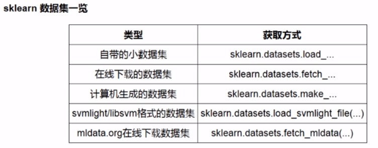
【sklearn的一般流程】数据的获取

1.生成回归数据 make_regression()

from sklearn.datasets import make_regression
X, y, coef = make_regression(n_samples=200, n_features=1, n_informative=1, n_targets=1,
                       bias = 0, effective_rank=None, noise = 20,
                        tail_strength=0,random_state=0, coef = True)

属性说明：

属性	默认值	说明
n_samples	int, optional (default=100)	样本数量
n_features	int, optional (default=100)	特征数量
n_informative	int, optional (default=10)	对回归有效的特征数量
n_targets	int, optional (default=1)	y的维度
bias	float, optional (default=0.0)	底层线性模型中的偏差项。相当于y的中位数
effective_rank	int or None, optional (default=None)	有效等级
noise	float, optional (default=0.0)	设置高斯噪声的标准偏差加到数据上。
shuffle	boolean, optional (default=True)	是否洗牌
coef	boolean, optional (default=False)	如果为真，则返回权重值
random_state	int,	设置随机种子

个人理解：
n_informative：该项为对本次回归有用的特征数量，举个例子，我们想要预测房价，手上的特征有：房子面积、房龄、地段和房主的名字，显然前3项特征时有效特征，而房主的名字属于无效特征，改变其值并不影响回归效果。这里的n_informative就是3，总特征数为4.
noise：其值是高斯分布的偏差值，其值越大数据越分散，其值越小数据越集中。
shuffle：设置是否洗牌，如果为False，会按照顺序创建样本，一般设置为True。

返回值：X ,y ,coef

效果图：

其coef（权重值） = 96.19

当设置更大的noise之后：

2.生成分类数据 make_classification()

from sklearn.datasets import make_classification
X, y = make_classification(n_samples=200, n_features=2, n_informative=2,n_redundant=0,
                           n_repeated=0, n_classes=2, n_clusters_per_class=1,random_state = 1)

plt.scatter(X[y == 0, 0], X[y == 0, 1], c = 'red', s = 100, label='0')
plt.scatter(X[y == 1, 0], X[y == 1, 1], c = 'blue', s = 100, label='1')
plt.scatter(X[y == 2, 0], X[y == 2, 1], c = 'green', s = 100, label='2')
plt.legend()
plt.show()

属性说明：

属性	默认值	说明
n_features	int, optional (default=20)	特征个数 >= n_informative（） + n_redundant + n_repeated
n_informative	int, optional (default=2)	有意义的特征数，对本次分类有利的特征数
n_redundant	int, optional (default=2)	冗余信息，informative特征的随机线性组合
n_repeated	int, optional (default=0)	重复信息，随机提取n_informative和n_redundant 特征
n_classes	int, optional (default=2)	分类类别
n_clusters_per_class	int, optional (default=2)	某一个类别是由几个cluster构成的（子类别）

返回值：X，y

效果图：

当将n_clusters_per_class 设置成2，即每个类中有2个子类别：

3. 生成二维线性不可分的数据集 make_circles()

from sklearn.datasets import make_circles
X, y = make_circles(n_samples=200, shuffle=True, noise = 0.05, factor=0.4, random_state=0)

plt.scatter(X[y == 0, 0], X[y == 0, 1], c = 'red', s = 100, label='0')
plt.scatter(X[y == 1, 0], X[y == 1, 1], c = 'blue', s = 100, label='1')
plt.scatter(X[y == 2, 0], X[y == 2, 1], c = 'green', s = 100, label='2')
plt.legend()
plt.show()

属性说明：

属性	默认值	说明
n_samples	int, optional (default=100)	样本的数量
shuffle	bool, optional (default=True)	是否洗牌
noise	double or None (default=None)	设置高斯噪声的标准偏差加到数据上。
random_state	int	随机种子
factor	double < 1 (default=.8)	外圈和内圈的比例

返回值：X，y

效果图：

当设置更大的factor时：

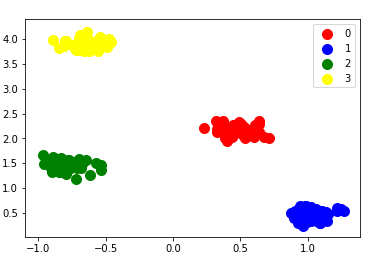
4. 生成用于聚类的数据集 make_blobs()

from sklearn.datasets import make_blobs
X, y = make_blobs(n_samples=200, n_features=2,centers = 4, cluster_std=0.5, center_box=(-5,5) ,random_state=0, shuffle= False)

plt.scatter(X[y == 0, 0], X[y == 0, 1], c = 'red', s = 100, label='0')
plt.scatter(X[y == 1, 0], X[y == 1, 1], c = 'blue', s = 100, label='1')
plt.scatter(X[y == 2, 0], X[y == 2, 1], c = 'green', s = 100, label='2')
plt.scatter(X[y == 3, 0], X[y == 3, 1], c = 'yellow', s = 100, label='3')
plt.legend()
plt.show()

属性说明：

属性	默认值	说明
n_samples	int, optional (default=100)	样本数量
n_features	int, optional (default=2)	特征数
centers	int or array of shape [n_centers, n_features], optional	中心数（类别数）
cluster_std	float or sequence of floats, optional (default=1.0)	每个集群的标准差
center_box	pair of floats (min, max), optional (default=(-10.0, 10.0))	每个样本的取值范围
random_state	int, RandomState instance or None, optional (default=None)	随机种子
shuffer	boolean, optional (default=True)	是否洗牌

返回值：X，y

效果图：

设置更小的cluster_std：

本节代码