深度学习笔记：简单神经网络

一.基础理论

二.反向链式法则推导

三.完整代码

import numpy as np

def sigmoid(x):
    # Sigmoid activation function: f(x) = 1 / (1 + e^(-x))
    return 1 / (1 + np.exp(-x))


def deriv_sigmoid(x):
    # Derivative of sigmoid: f'(x) = f(x) * (1 - f(x))
    fx = sigmoid(x)
    return fx * (1 - fx)


def mse_loss(y_true, y_pred):
    # y_true and y_pred are numpy arrays of the same length
    return ((y_true - y_pred) ** 2).mean()


class OurNeuralNetwork():
    """
    A neural network with:
      - 2 inputs
      - a hidden layer with 2 neurons (h1, h2)
      - an output layer with 1 neuron (o1)

    *** DISCLAIMER ***
    The code below is intend to be simple and educational, NOT optimal.
    Real neural net code looks nothing like this. Do NOT use this code.
    Instead, read/run it to understand how this specific network works.
    """

    def __init__(self):
        # weights 权值
        self.w1 = np.random.normal()
        self.w2 = np.random.normal()
        self.w3 = np.random.normal()
        self.w4 = np.random.normal()
        self.w5 = np.random.normal()
        self.w6 = np.random.normal()
        # biases
        self.b1 = np.random.normal()
        self.b2 = np.random.normal()
        self.b3 = np.random.normal()

    # 预测时正向计算
    def feedforward(self, x):
        # x is a numpy array with 2 elements, for example [input1, input2]， x有两个特征值，x0(体重), x1(高度)
        h1 = sigmoid(self.w1 * x[0] + self.w2 * x[1] + self.b1)
        h2 = sigmoid(self.w3 * x[0] + self.w4 * x[1] + self.b2)
        o1 = sigmoid(self.w5 * h1 + self.w6 * h2 + self.b3)
        return o1

    def train(self, data, all_y_trues):
        """
        - data is a (n x 2) numpy array, n = # samples in the dataset.
        - all_y_trues is a numpy array with n elements.
        Elements in all_y_trues correspond to those in data.
        """
        learn_rate = 0.1
        epochs = 1000  # number of times to loop through the entire dataset

        for epoch in range(epochs):
            for x, y_true in zip(data, all_y_trues):
                # - - - Do a feedforward (we'll need these values later)
                sum_h1 = self.w1 * x[0] + self.w2 * x[1] + self.b1
                h1 = sigmoid(sum_h1)

                sum_h2 = self.w3 * x[0] + self.w4 * x[1] + self.b2
                h2 = sigmoid(sum_h2)

                sum_o1 = self.w5 * h1 + self.w6 * h2 + self.b3
                o1 = sigmoid(sum_o1)
                y_pred = o1

                # - - - Calculate partial derivatives.
                # - - - Naming: d_L_d_w1 represents "partial L / partial w1"
                d_L_d_ypred = -2 * (y_true - y_pred)

                # Neuron o1，o1的求导, 从输出层到隐藏层
                # 先求w5, w6, b3
                d_ypred_d_w5 = h1 * deriv_sigmoid(sum_o1)
                d_ypred_d_w6 = h2 * deriv_sigmoid(sum_o1)
                d_ypred_d_b3 = deriv_sigmoid(sum_o1)

                # 再求h1, h2
                d_ypred_d_h1 = self.w5 * deriv_sigmoid(sum_o1)
                d_ypred_d_h2 = self.w6 * deriv_sigmoid(sum_o1)

                # Neuron h1，h1作为输入求w1, w2，从隐藏层到输入层
                d_h1_d_w1 = x[0] * deriv_sigmoid(sum_h1)        # dz * x
                d_h1_d_w2 = x[1] * deriv_sigmoid(sum_h1)
                d_h1_d_b1 = deriv_sigmoid(sum_h1)

                # Neuron h2, h2作为输入求w3, w4
                d_h2_d_w3 = x[0] * deriv_sigmoid(sum_h2)
                d_h2_d_w4 = x[1] * deriv_sigmoid(sum_h2)
                d_h2_d_b2 = deriv_sigmoid(sum_h2)

                # - - - update weights and biases, 梯度下降
                # Neuron o1
                self.w5 -= learn_rate * d_L_d_ypred * d_ypred_d_w5
                self.w6 -= learn_rate * d_L_d_ypred * d_ypred_d_w6
                self.b3 -= learn_rate * d_L_d_ypred * d_ypred_d_b3

                # Neuron h1
                self.w1 -= learn_rate * d_L_d_ypred * d_ypred_d_h1 * d_h1_d_w1
                self.w2 -= learn_rate * d_L_d_ypred * d_ypred_d_h1 * d_h1_d_w2
                self.b1 -= learn_rate * d_L_d_ypred * d_ypred_d_h1 * d_h1_d_b1

                # Neuron h2
                self.w3 -= learn_rate * d_L_d_ypred * d_ypred_d_h2 * d_h2_d_w3
                self.w4 -= learn_rate * d_L_d_ypred * d_ypred_d_h2 * d_h2_d_w4
                self.b2 -= learn_rate * d_L_d_ypred * d_ypred_d_h2 * d_h2_d_b2

            # - - - Calculate total loss at the end of each epoch
            if epoch % 10 == 0:
                y_preds = np.apply_along_axis(self.feedforward, 1, data)
                loss = mse_loss(all_y_trues, y_preds)
                print("Epoch %d loss: %.3f", (epoch, loss))


# Define dataset
data = np.array([
    [-2, -1],       # Alice
    [25, 6],        # Bob
    [17, 4],        # Charlie
    [-15, -6]       # diana
])

# 0 男， 1 女
all_y_trues = np.array([
    1,  # Alice
    0,  # Bob
    0,  # Charlie
    1   # diana
])

# Train our neural network!
network = OurNeuralNetwork()
network.train(data, all_y_trues)

# Make some predictions
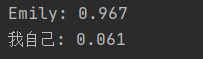
emily = np.array([-7, -3]) # 128 pounds, 63 inches
我自己 = np.array([2, 4])  # 155 pounds, 68 inches
print("Emily: %.3f" % network.feedforward(emily)) # 0.951 - F
print("Frank: %.3f" % network.feedforward(frank)) # 0.039 - M