遗传算法(GA)学习以及python实现(附C++TSP)

前些日子，我用C++手写代码实现了遗传算法解决TSP问题，C++太过于繁琐而且写的也不是很好，解决了以下问题:

问题：给定平面上20个点的名称与坐标，两个点之间的距离为它们的欧几里得距离。求一条路径，刚好经过每个点1次，使其路径长度最短。
参数设定如下：
种群大小：M=50
最大代数：G=1000
交叉率：pc=1pc=1,交叉率为1能保证种群的充分进化
变异率：pm=0.1pm=0.1,一般而言，变异发生的可能性较小
在该问题中，每一条路径就是所谓的染色体（解的编码），每条路径的长度就是该个体的适应性（路径长度越短，适应性越强）。交叉操作就是选择两条路径，取一个分界点k，将两条路径分别以分界点k分成前后两段，并且将两条路径重新组合得到新的两条路径。这里的交叉操作蕴含了变异操作，但是能够让子代继承父代的优良特性。变异操作也是实现群体多样性的一种手段，也是全局寻优的保证，具体实现为，按照给定的变异率，对选定的变异的个体，随机的选取三个整数u

这里原理就不具体阐述了，GA是一种基于自然选择原理和自然遗传机制的搜索(寻优)算法，它是模拟自然界中的生命进化机制，在人工系统中实现特定目标的优化。遗传算法的实质是通过群体搜索技术，根据适者生存的原则逐代进化，最终得到最优解或准最优解。它必须做以下操作:初始群体的产生、求每一个体的适应度、根据适者生存的原则选择优良个体、被选出的优良个体两两配对，通过随机交叉其染色体的基因并随机变异某些染色体的基因后生成下一代群体，按此方法使群体逐代进化，直到满足进化终止条件。
以下是解决的C++代码:

#include <iostream>
#include <algorithm>
#include <fstream>
#include <vector>
#include <ctime>
#include "cmath"
using namespace std;
const int maxn = 100;
struct Point{
    string name;
    double x,y;
    int i;
};
vector<Point> p;
double d[maxn][maxn];
int n;
double sum = 0;

double dist(Point a, Point b) { //计算两点距离
    return sqrt((a.x - b.x) * (a.x - b.x) + (a.y - b.y) * (a.y - b.y));
}
double get_sum(vector<Point> a){
    double sum = 0;
    for (int i = 1; i < a.size(); i++) {
        sum += d[a[i].i][a[i - 1].i];
    }
    sum += d[a[0].i][a[a.size()-1].i];
    return sum;
}

void init(){
    srand((unsigned)time(NULL)); //设置随机数种子
    ifstream ifs;
    ifs.open("input.txt");
    p.clear();
    ifs>>n;
    for (int i=0; i<n; ++i){
        Point t;
        ifs>>t.name>>t.x>>t.y;
        t.i = i;
        p.push_back(t);
    }
    for(int i=0; i<n; ++i){
        for(int j=i+1;j<n;++j){
            d[i][j] = d[j][i] = dist(p[i], p[j]);
        }
    }
    sum = get_sum(p);
}

void show() { //显示当前结果
    cout << "路径长度: " << sum << endl;
    cout << "路径:";
    for (int i = 0; i < n; i++)
        cout << ' ' << p[i].name;
    puts("");
}
int w = 100;                  //限定种群只能活100个个体
vector<vector<Point>> group; //种群，也就是染色体列表

void Improve_Circle() { //改良圈法得到初始序列
    vector<Point> cur = p;
    for (int t = 0; t < w; t++) {     //重复50次
        for (int i = 0; i < n; i++) { //构造随机顺序
            int j = rand() % n;
            swap(cur[i], cur[j]);
        }
        int flag = 1;
        while (flag) {
            flag = 0;
            //不断选取uv子串，尝试倒置uv子串的顺序后解是否更优，如果更优则变更
            for (int u = 1; u < n - 2; u++) {
                for (int v = u + 1; v < n - 1; v++) {
                    if (d[cur[u].i][cur[v + 1].i] + d[cur[u - 1].i][cur[v].i] <
                        d[cur[u].i][cur[u - 1].i] + d[cur[v].i][cur[v + 1].i]) {
                        for (int k = u; k <= (u + v) / 2; k++) {
                            swap(cur[k], cur[v - (k - u)]);
                            flag = 1;
                        }
                    }
                }
            }
        }
        group.push_back(cur);
        double cur_sum = get_sum(cur);
        if (cur_sum < sum) {
            sum = cur_sum;
            p = cur;
        }
    }
}

vector<int> get_randPerm(int n) { //返回一个随机序列
    vector<int> c;
    for (int i = 0; i < n; i++) {
        c.push_back(i);
    }
    for (int i = 0; i < n; i++) {
        swap(c[i], c[rand() % n]);
    }
    return c;
}

//排序时用到的比较函数
bool cmp(vector<Point> a, vector<Point> b){
    return get_sum(a) < get_sum(b);
}
int gen = 400; //一共进行400代的进化选择
int c[maxn];
double rate = 0.1; //变异率

void genetic_algorithm() { //遗传算法
    vector<vector<Point>> A = group, B, C;
    // A：当前代的种群  B:交配产生的子代  C：变异产生的子代
    for (int t = 0; t < gen; t++) {
        B = A;
        vector<int> c = get_randPerm(A.size());
        for (int i = 0; i + 1 < c.size(); i += 2) {
            int F = rand() % n; //基因划分分界点
            int u=c[i],v=c[i+1];
            for (int j = F; j < n;j++) { //交换随机选的2个个体的基因后半段，也就是交配
                swap(B[u][j], B[v][j]);
            }
            //交换后可能发生冲突，需要解除冲突
            //保留F前面的部分不变，F后面的部分有冲突则交换
            int num1[1000]={0},num2[1000]={0};
            for(int j=0;j<n;j++){
                num1[B[u][j].i]++;
                num2[B[v][j].i]++;
            }
            vector<Point> v1;
            vector<Point> v2;
            for(int j=0;j<n;j++){
                if(num1[B[u][j].i]==2){
                    v1.push_back(B[u][j]);
                }
            }
            for(int j=0;j<n;j++){
                if(num2[B[v][j].i]==2){
                    v2.push_back(B[v][j]);
                }
            }
            int p1=0,p2=0;
            for(int j=F;j<n;j++){
                if(num1[B[u][j].i]==2){
                    B[u][j]=v2[p2++];
                }
                if(num2[B[v][j].i]==2){
                    B[v][j]=v1[p1++];
                }
            }
        }
        C.clear();
        int flag=1;
        for (int i = 0; i < A.size(); i++) {
            if (rand() % 100 >= rate * 100)
                continue;
            //对于变异的个体,取3个点u<v<w,把子串[u,v]插到w后面
            int u, v, w;
            u = rand() % n;
            do {
                v = rand() % n;
            } while (u == v);
            do {
                w = rand() % n;
            } while (w == u || w == v);
            if (u > v)
                swap(u, v);
            if (v > w)
                swap(v, w);
            if (u > v)
                swap(u, v);

            vector<Point> vec;
            for (int j = 0; j < u; j++)
                vec.push_back(A[i][j]);
            for (int j = v; j < w; j++)
                vec.push_back(A[i][j]);
            for (int j = u; j < v; j++)
                vec.push_back(A[i][j]);
            for (int j = w; j < n; j++)
                vec.push_back(A[i][j]);
            C.push_back(vec);
        }
        //合并A，B，C
        for (int i = 0; i < B.size(); i++) {
            A.push_back(B[i]);
        }
        for (int i = 0; i < C.size(); i++) {
            A.push_back(C[i]);
        }
        sort(A.begin(), A.end(), cmp); //从小到大排序
        vector<vector<Point>> new_A;
        for (int i = 0; i < w; i++) {
            new_A.push_back(A[i]);
        }
        A = new_A;
    }
    group = A;
    sum = get_sum(group[0]);
    p = group[0];
}

int main(){
    init();
    cout << "初始";
    show();
    cout << "改良圈法";
    Improve_Circle();
    show();
    cout << "遗传算法";
    genetic_algorithm();
    show();
    exit(0);
}

在数学建模学习的时候重温GA算法，发现了一位大佬写的非常方便的包scikit-opt

pip install scikit-opt

把源代码中的sko文件夹下载下来放本地也调用

这个包里面有PSO、GA、SA算法调用，这里主要讲GA算法的使用:

遗传算法基本使用并且画图

import numpy as np


def schaffer(p):
    '''
    This function has plenty of local minimum, with strong shocks
    global minimum at (0,0) with value 0
    https://en.wikipedia.org/wiki/Test_functions_for_optimization
    '''
    x1, x2 = p
    part1 = np.square(x1) - np.square(x2)
    part2 = np.square(x1) + np.square(x2)
    return 0.5 + (np.square(np.sin(part1)) - 0.5) / np.square(1 + 0.001 * part2)


# %%
from sko.GA import GA

ga = GA(func=schaffer, n_dim=2, size_pop=50, max_iter=800, prob_mut=0.001, lb=[-1, -1], ub=[1, 1], precision=1e-7)
best_x, best_y = ga.run()
print('best_x:', best_x, '\n', 'best_y:', best_y)
# %% Plot the result
import pandas as pd
import matplotlib.pyplot as plt

Y_history = pd.DataFrame(ga.all_history_Y)
fig, ax = plt.subplots(2, 1)
ax[0].plot(Y_history.index, Y_history.values, '.', color='red')
Y_history.min(axis=1).cummin().plot(kind='line')
plt.show()

也可以使用lambda表达式形式定义变量
在多维优化时，想让哪个变量限制为整数，就设定 precision 为 整数 即可。
例如，我想让我的自定义函数 schaffer 的某些变量限制为整数+浮点数（分别是隔2个，隔1个，浮点数），那么就设定 precision=[2, 1, 1e-7]

from sko.GA import GA

schaffer = lambda x: (x[0] - 1) ** 2 + (x[1] - 0.05) ** 2 + x[2] ** 2
ga = GA(func=schaffer, n_dim=3, max_iter=500, lb=[-1, -1, -1], ub=[5, 1, 1], precision=[2, 1, 1e-7])
best_x, best_y = ga.run()
print('best_x:', best_x, '\n', 'best_y:', best_y)

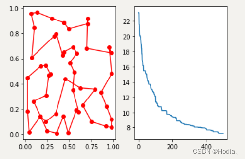
python遗传算法解决TSP问题

这里使用欧几里得距离(euclidean)求解

import numpy as np
from scipy import spatial
import matplotlib.pyplot as plt

num_points = 50

points_coordinate = np.random.rand(num_points, 2)  # generate coordinate of points
distance_matrix = spatial.distance.cdist(points_coordinate, points_coordinate, metric='euclidean')


def cal_total_distance(routine):
    '''The objective function. input routine, return total distance.
    cal_total_distance(np.arange(num_points))
    '''
    num_points, = routine.shape
    return sum([distance_matrix[routine[i % num_points], routine[(i + 1) % num_points]] for i in range(num_points)])


# %% do GA

from sko.GA import GA_TSP

ga_tsp = GA_TSP(func=cal_total_distance, n_dim=num_points, size_pop=50, max_iter=500, prob_mut=1)
best_points, best_distance = ga_tsp.run()

# %% plot
fig, ax = plt.subplots(1, 2)
best_points_ = np.concatenate([best_points, [best_points[0]]])
best_points_coordinate = points_coordinate[best_points_, :]
ax[0].plot(best_points_coordinate[:, 0], best_points_coordinate[:, 1], 'o-r')
ax[1].plot(ga_tsp.generation_best_Y)
plt.show()

结果如下

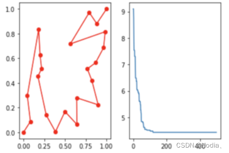
TSP算法限定起始点

固定起点和终点要求路径不闭合（因为如果路径是闭合的，固定与不固定结果实际上是一样的）

假设你的起点和终点坐标指定为(0, 0) 和 (1, 1)，这样构建目标函数

• 起点和终点不参与优化。假设共有n+2个点，优化对象是中间n个点
• 目标函数（总距离）按实际去写。

import numpy as np
from scipy import spatial
import matplotlib.pyplot as plt

num_points = 20

points_coordinate = np.random.rand(num_points, 2)  # generate coordinate of points
start_point=[[0,0]]
end_point=[[1,1]]
points_coordinate=np.concatenate([points_coordinate,start_point,end_point])
distance_matrix = spatial.distance.cdist(points_coordinate, points_coordinate, metric='euclidean')


def cal_total_distance(routine):
    '''The objective function. input routine, return total distance.
    cal_total_distance(np.arange(num_points))
    '''
    num_points, = routine.shape
    # start_point,end_point 本身不参与优化。给一个固定的值，参与计算总路径
    routine = np.concatenate([[num_points], routine, [num_points+1]])
    return sum([distance_matrix[routine[i], routine[i + 1]] for i in range(num_points+2-1)])

正常运行并画图：

from sko.GA import GA_TSP

ga_tsp = GA_TSP(func=cal_total_distance, n_dim=num_points, size_pop=50, max_iter=500, prob_mut=1)
best_points, best_distance = ga_tsp.run()


fig, ax = plt.subplots(1, 2)
best_points_ = np.concatenate([[num_points],best_points, [num_points+1]])
best_points_coordinate = points_coordinate[best_points_, :]
ax[0].plot(best_points_coordinate[:, 0], best_points_coordinate[:, 1], 'o-r')
ax[1].plot(ga_tsp.generation_best_Y)
plt.show()

结果如下: