TensorFlow 全连接网络实现

1**神经网络**是一种数学模型，大量的神经元相连接并进行计算，用来对输入和输出间复杂的关系进行建模。

神经网络训练，通过大量数据样本，对比正确答案和模型输出之间的区别（梯度），然后把这个区别（梯度）反向的传递回去，对每个相应的神经元进行一点点的改变。那么下一次在训练的时候就可以用已经改进一点点的神经元去得到稍微准确一点的结果。

基于TensorFlow实现一个简单的神经网络。

结构图

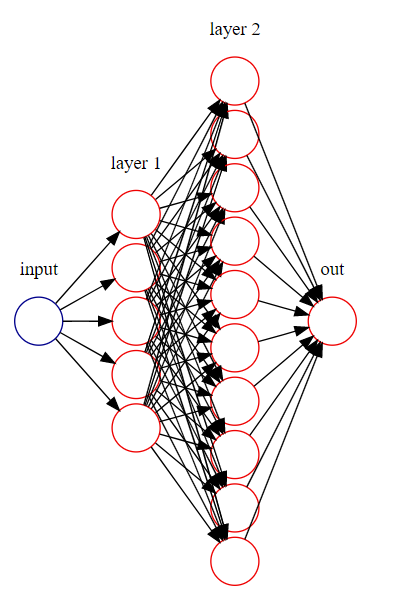
搭建神经网络图

1. 准备训练数据

导入相应的包：

import tensorflow as tf
import numpy as np
import matplotlib.pyplot as plt
   
   
1
2
3

准备训练数据：

x_data = np.linspace(-1, 1, 300, dtype=np.float32)[:, np.newaxis]
noise = np.random.normal(0, 0.05, x_data.shape).astype(np.float32)
y_data = 2 * np.power(x_data, 3) + np.power(x_data, 2) + noise
   
   
1
2
3

2. 定义网络结构

定义占位符：

xs = tf.placeholder(tf.float32, [None, 1])
ys = tf.placeholder(tf.float32, [None, 1])
   
   
1
2

定义神经层：隐藏层和预测层

# 隐层1
Weights1 = tf.Variable(tf.random_normal([1, 5]))
biases1 = tf.Variable(tf.zeros([1, 5]) + 0.1)
Wx_plus_b1 = tf.matmul(xs, Weights1) + biases1
l1 = tf.nn.relu(Wx_plus_b1)
# 隐层2
Weights2 = tf.Variable(tf.random_normal([5, 10]))
biases2 = tf.Variable(tf.zeros([1, 10]) + 0.1)
Wx_plus_b2 = tf.matmul(l1, Weights2) + biases2
l2 = tf.nn.relu(Wx_plus_b2)
# 输出层
Weights3 = tf.Variable(tf.random_normal([10, 1]))
biases3 = tf.Variable(tf.zeros([1, 1]) + 0.1)
prediction = tf.matmul(l2, Weights3) + biases3
   
   
1
2
3
4
5
6
7
8
9
10
11
12
13
14

3. 定义 loss 表达式

这里采用均方差（mean squared error）：

MAE(y,y^)=1nsamples∑i=1n(yi−yi^)2” role=”presentation” style=”text-align: center; position: relative;”>MAE(y,y^)=1nsamples∑i=1n(yi−yi^)2MAE(y,y^)=1nsamples∑i=1n(yi−yi^)2

MAE(y,\hat{y}) = \frac{1}{n_{samples}} \sum_{i=1}^n (y_i - \hat{y_i})^2

loss = tf.reduce_mean(tf.reduce_sum(tf.square(ys - prediction), reduction_indices=[1]))
   
   
1

4. optimizer

即训练的优化策略，一般有梯度下降（GradientDescentOptimizer）、AdamOptimizer等。.minimize(loss)是让 loss 达到最小。

train_step = tf.train.AdamOptimizer(0.1).minimize(loss)
   
   
1

训练

# 初始化所有变量
init = tf.global_variables_initializer()
# 激活会话
with tf.Session() as sess:
    sess.run(init)
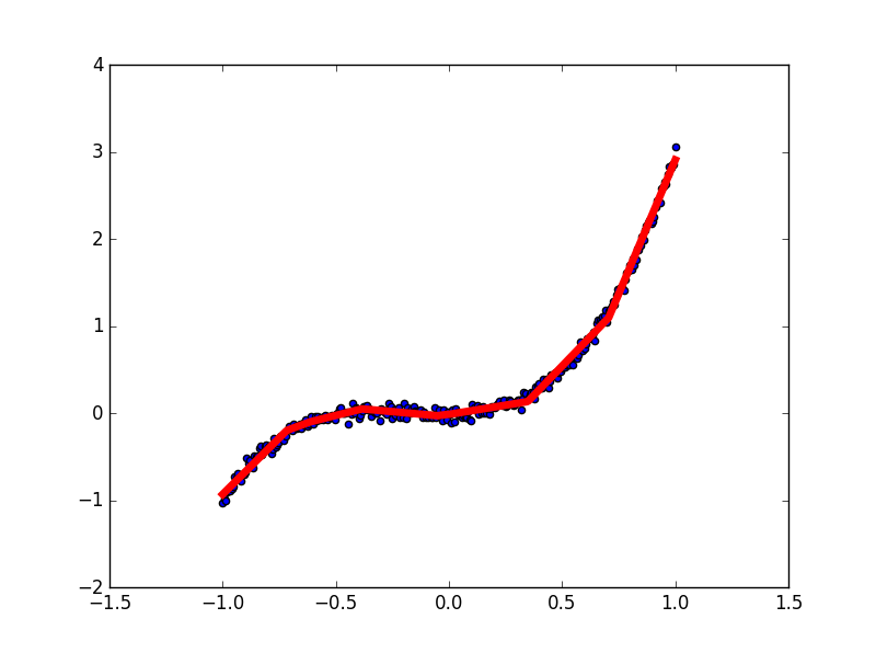
    # 绘制原始x-y散点图。
    fig = plt.figure()
    ax = fig.add_subplot(1, 1, 1)
    ax.scatter(x_data, y_data)
    plt.ion()
    plt.show()
    # 迭代次数 = 10000
    for i in range(10000):
        # 训练
        sess.run(train_step, feed_dict={xs: x_data, ys: y_data})
        # 每50步绘图并打印输出。
        if i % 50 == 0:
            # 可视化模型输出的结果。
            try:
                ax.lines.remove(lines[0])
            except Exception:
                pass
            prediction_value = sess.run(prediction, feed_dict={xs: x_data})
            # 绘制模型预测值。
            lines = ax.plot(x_data, prediction_value, 'r-', lw=5)
            plt.pause(1)
            # 打印损失
            print(sess.run(loss, feed_dict={xs: x_data, ys: y_data}))
   
   
1
2
3
4
5
6
7
8
9
10
11
12
13
14
15
16
17
18
19
20
21
22
23
24
25
26
27
28

最终结果

最终损失：0.0026713（不同的初始化可能会有不同）

GitHub完整代码：FullConnectedNetwork.py

Reference

1. youtube 上的课程

   ​

        <link rel="stylesheet" href="https://csdnimg.cn/release/phoenix/template/css/markdown_views-ea0013b516.css">
            </div>