压缩感知重构算法之压缩感知匹配追踪（CoSaMp）

最新推荐文章于 2023-02-25 00:58:02 发布

yuehuihui00

最新推荐文章于 2023-02-25 00:58:02 发布

阅读量1.7k

点赞数

压缩感知重构算法之压缩采样匹配追踪(CoSaMP)

转载自彬彬有礼的专栏

题目：压缩感知重构算法之压缩采样匹配追踪（CoSaMP）

压缩采样匹配追踪(CompressiveSampling MP)是D. Needell继ROMP之后提出的又一个具有较大影响力的重构算法。CoSaMP也是对OMP的一种改进，每次迭代选择多个原子，除了原子的选择标准之外，它有一点不同于ROMP：ROMP每次迭代已经选择的原子会一直保留，而CoSaMP每次迭代选择的原子在下次迭代中可能会被抛弃。

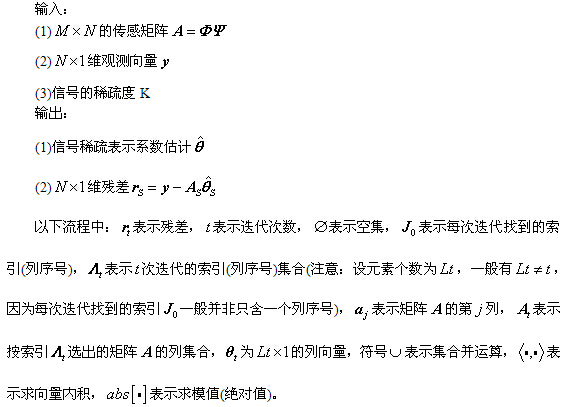
0、符号说明如下：

压缩观测y=Φx，其中y为观测所得向量M×1，x为原信号N×1（M<<N）。x一般不是稀疏的，但在某个变换域Ψ是稀疏的，即x=Ψθ，其中θ为K稀疏的，即θ只有K个非零项。此时y=ΦΨθ，令A=ΦΨ，则y=Aθ。

(1) y为观测所得向量，大小为M×1

(2)x为原信号，大小为N×1

(3)θ为K稀疏的，是信号在x在某变换域的稀疏表示

(4) Φ称为观测矩阵、测量矩阵、测量基，大小为M×N

(5) Ψ称为变换矩阵、变换基、稀疏矩阵、稀疏基、正交基字典矩阵，大小为N×N

(6)A称为测度矩阵、传感矩阵、CS信息算子，大小为M×N

上式中，一般有K<<M<<N，后面三个矩阵各个文献的叫法不一，以后我将Φ称为测量矩阵、将Ψ称为稀疏矩阵、将A称为传感矩阵。

注意：这里的稀疏表示模型为x=Ψθ，所以传感矩阵A=ΦΨ；而有些文献中稀疏模型为θ=Ψx，而一般Ψ为Hermite矩阵(实矩阵时称为正交矩阵)，所以Ψ^-1=Ψ^H (实矩阵时为Ψ^-1=Ψ^T)，即x=Ψ^Hθ，所以传感矩阵A=ΦΨ^H，例如沙威的OMP例程中就是如此。

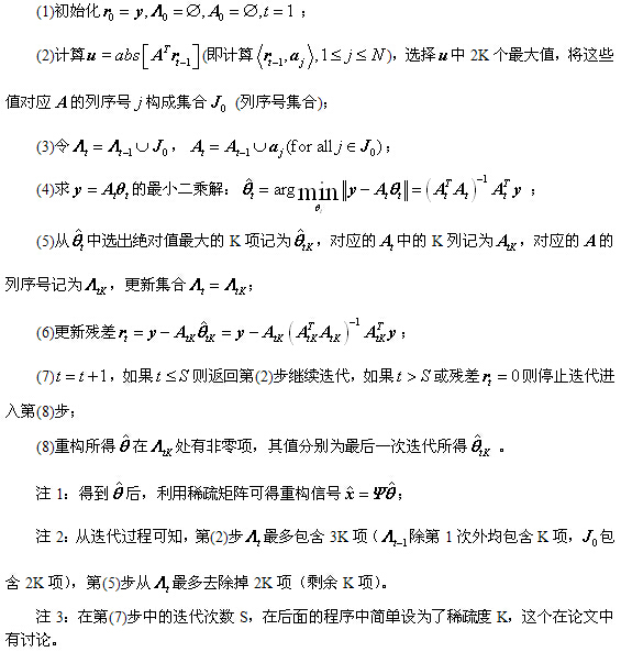
1、CoSaMP重构算法流程：

2、压缩采样匹配追踪(CoSaOMP)Matlab代码(CS_CoSaMP.m)

代码参考了文献[5]中的Demo_CS_CoSaMP.m，也可参考文献[6]，或者文献[7]中的cosamp.m。值得一提的是文献[5]的所有代码都挺不错的，从代码注释中可以得知作者是ustc的ChengfuHuo，百度一下可知是中国科技大学的霍承富博士，已于2012年6月毕业，博士论文题目是《超光谱遥感图像压缩技术研究》，向这位学长致敬！（虽然不是一个学校的）

2015-05-13更新：

[plain] view plain copy

print ?

function [ theta ] = CS_CoSaMP( y,A,K )
%CS_CoSaOMP Summary of this function goes here
%Created by jbb0523@@2015-04-29
%Version: 1.1 modified by jbb0523 @2015-05-09
% Detailed explanation goes here
% y = Phi * x
% x = Psi * theta
% y = Phi*Psi * theta
% 令 A = Phi*Psi, 则y=A*theta
% K is the sparsity level
% 现在已知y和A，求theta
% Reference:Needell D，Tropp J A．CoSaMP：Iterative signal recovery from
% incomplete and inaccurate samples[J]．Applied and Computation Harmonic
% Analysis，2009，26：301-321.
[y_rows,y_columns] = size(y);
if y_rows<y_columns
y = y';%y should be a column vector
end
[M,N] = size(A);%传感矩阵A为M*N矩阵
theta = zeros(N,1);%用来存储恢复的theta(列向量)
Pos_theta = [];%用来迭代过程中存储A被选择的列序号
r_n = y;%初始化残差(residual)为y
for kk=1:K%最多迭代K次
%(1) Identification
product = A'*r_n;%传感矩阵A各列与残差的内积
[val,pos]=sort(abs(product),'descend');
Js = pos(1:2*K);%选出内积值最大的2K列
%(2) Support Merger
Is = union(Pos_theta,Js);%Pos_theta与Js并集
%(3) Estimation
%At的行数要大于列数，此为最小二乘的基础(列线性无关)
if length(Is)<=M
At = A(:,Is);%将A的这几列组成矩阵At
else%At的列数大于行数，列必为线性相关的,At'*At将不可逆
if kk == 1
theta_ls = 0;
end
break;%跳出for循环
end
%y=At*theta，以下求theta的最小二乘解(Least Square)
theta_ls = (At'*At)^(-1)*At'*y;%最小二乘解
%(4) Pruning
[val,pos]=sort(abs(theta_ls),'descend');
%(5) Sample Update
Pos_theta = Is(pos(1:K));
theta_ls = theta_ls(pos(1:K));
%At(:,pos(1:K))*theta_ls是y在At(:,pos(1:K))列空间上的正交投影
r_n = y - At(:,pos(1:K))*theta_ls;%更新残差
if norm(r_n)<1e-6%Repeat the steps until r=0
break;%跳出for循环
end
end
theta(Pos_theta)=theta_ls;%恢复出的theta
end

function [ theta ] = CS_CoSaMP( y,A,K )
%CS_CoSaOMP Summary of this function goes here
%Created by jbb0523@@2015-04-29
%Version: 1.1 modified by jbb0523 @2015-05-09
%   Detailed explanation goes here
%   y = Phi * x
%   x = Psi * theta
%	y = Phi*Psi * theta
%   令 A = Phi*Psi, 则y=A*theta
%   K is the sparsity level
%   现在已知y和A，求theta
%   Reference:Needell D，Tropp J A．CoSaMP：Iterative signal recovery from
%   incomplete and inaccurate samples[J]．Applied and Computation Harmonic 
%   Analysis，2009，26：301-321.
    [y_rows,y_columns] = size(y);
    if y_rows<y_columns
        y = y';%y should be a column vector
    end
    [M,N] = size(A);%传感矩阵A为M*N矩阵
    theta = zeros(N,1);%用来存储恢复的theta(列向量)
    Pos_theta = [];%用来迭代过程中存储A被选择的列序号
    r_n = y;%初始化残差(residual)为y
    for kk=1:K%最多迭代K次
        %(1) Identification
        product = A'*r_n;%传感矩阵A各列与残差的内积
        [val,pos]=sort(abs(product),'descend');
        Js = pos(1:2*K);%选出内积值最大的2K列
        %(2) Support Merger
        Is = union(Pos_theta,Js);%Pos_theta与Js并集
        %(3) Estimation
        %At的行数要大于列数，此为最小二乘的基础(列线性无关)
        if length(Is)<=M
            At = A(:,Is);%将A的这几列组成矩阵At
        else%At的列数大于行数，列必为线性相关的,At'*At将不可逆
            if kk == 1
                theta_ls = 0;
            end
            break;%跳出for循环
        end
        %y=At*theta，以下求theta的最小二乘解(Least Square)
        theta_ls = (At'*At)^(-1)*At'*y;%最小二乘解
        %(4) Pruning
        [val,pos]=sort(abs(theta_ls),'descend');
        %(5) Sample Update
        Pos_theta = Is(pos(1:K));
        theta_ls = theta_ls(pos(1:K));
        %At(:,pos(1:K))*theta_ls是y在At(:,pos(1:K))列空间上的正交投影
        r_n = y - At(:,pos(1:K))*theta_ls;%更新残差 
        if norm(r_n)<1e-6%Repeat the steps until r=0
            break;%跳出for循环
        end
    end
    theta(Pos_theta)=theta_ls;%恢复出的theta
end

原先的版本：

[plain] view plain copy

print ?

function [ theta ] = CS_CoSaMP( y,A,K )
%CS_CoSaMP Summary of this function goes here
%Version: 1.0 written by jbb0523 @2015-04-29
% Detailed explanation goes here
% y = Phi * x
% x = Psi * theta
% y = Phi*Psi * theta
% 令 A = Phi*Psi, 则y=A*theta
% K is the sparsity level
% 现在已知y和A，求theta
% Reference:Needell D，Tropp J A．CoSaMP：Iterative signal recovery from
% incomplete and inaccurate samples[J]．Applied and Computation Harmonic
% Analysis，2009，26：301-321.
[y_rows,y_columns] = size(y);
if y_rows<y_columns
y = y';%y should be a column vector
end
[M,N] = size(A);%传感矩阵A为M*N矩阵
theta = zeros(N,1);%用来存储恢复的theta(列向量)
Pos_theta = [];%用来迭代过程中存储A被选择的列序号
r_n = y;%初始化残差(residual)为y
for kk=1:K%最多迭代K次
%(1) Identification
product = A'*r_n;%传感矩阵A各列与残差的内积
[val,pos]=sort(abs(product),'descend');
Js = pos(1:2*K);%选出内积值最大的2K列
%(2) Support Merger
Is = union(Pos_theta,Js);%Pos_theta与Js并集
%(3) Estimation
%At的行数要大于列数，此为最小二乘的基础(列线性无关)
if length(Is)<=M
At = A(:,Is);%将A的这几列组成矩阵At
else%At的列数大于行数，列必为线性相关的,At'*At将不可逆
break;%跳出for循环
end
%y=At*theta，以下求theta的最小二乘解(Least Square)
theta_ls = (At'*At)^(-1)*At'*y;%最小二乘解
%(4) Pruning
[val,pos]=sort(abs(theta_ls),'descend');
%(5) Sample Update
Pos_theta = Is(pos(1:K));
theta_ls = theta_ls(pos(1:K));
%At(:,pos(1:K))*theta_ls是y在At(:,pos(1:K))列空间上的正交投影
r_n = y - At(:,pos(1:K))*theta_ls;%更新残差
if norm(r_n)<1e-6%Repeat the steps until r=0
break;%跳出for循环
end
end
theta(Pos_theta)=theta_ls;%恢复出的theta
end

function [ theta ] = CS_CoSaMP( y,A,K )
%CS_CoSaMP Summary of this function goes here
%Version: 1.0 written by jbb0523 @2015-04-29
%   Detailed explanation goes here
%   y = Phi * x
%   x = Psi * theta
%	y = Phi*Psi * theta
%   令 A = Phi*Psi, 则y=A*theta
%   K is the sparsity level
%   现在已知y和A，求theta
%   Reference:Needell D，Tropp J A．CoSaMP：Iterative signal recovery from
%   incomplete and inaccurate samples[J]．Applied and Computation Harmonic 
%   Analysis，2009，26：301-321.
    [y_rows,y_columns] = size(y);
    if y_rows<y_columns
        y = y';%y should be a column vector
    end
    [M,N] = size(A);%传感矩阵A为M*N矩阵
    theta = zeros(N,1);%用来存储恢复的theta(列向量)
    Pos_theta = [];%用来迭代过程中存储A被选择的列序号
    r_n = y;%初始化残差(residual)为y
    for kk=1:K%最多迭代K次
        %(1) Identification
        product = A'*r_n;%传感矩阵A各列与残差的内积
        [val,pos]=sort(abs(product),'descend');
        Js = pos(1:2*K);%选出内积值最大的2K列
        %(2) Support Merger
        Is = union(Pos_theta,Js);%Pos_theta与Js并集
        %(3) Estimation
        %At的行数要大于列数，此为最小二乘的基础(列线性无关)
        if length(Is)<=M
            At = A(:,Is);%将A的这几列组成矩阵At
        else%At的列数大于行数，列必为线性相关的,At'*At将不可逆
            break;%跳出for循环
        end
        %y=At*theta，以下求theta的最小二乘解(Least Square)
        theta_ls = (At'*At)^(-1)*At'*y;%最小二乘解
        %(4) Pruning
        [val,pos]=sort(abs(theta_ls),'descend');
        %(5) Sample Update
        Pos_theta = Is(pos(1:K));
        theta_ls = theta_ls(pos(1:K));
        %At(:,pos(1:K))*theta_ls是y在At(:,pos(1:K))列空间上的正交投影
        r_n = y - At(:,pos(1:K))*theta_ls;%更新残差 
        if norm(r_n)<1e-6%Repeat the steps until r=0
            break;%跳出for循环
        end
    end
    theta(Pos_theta)=theta_ls;%恢复出的theta
end

在程序主循环的(3)Estimation部分增加了以下几行代码，以使函数运行更加稳定：

[plain] view plain copy

print ?

if kk == 1
theta_ls = 0;
end

            if kk == 1
                theta_ls = 0;
            end

3、CoSaMP单次重构测试代码

以下测试代码基本与OMP单次重构测试代码一样。

[plain] view plain copy

print ?

%压缩感知重构算法测试
clear all;close all;clc;
M = 64;%观测值个数
N = 256;%信号x的长度
K = 12;%信号x的稀疏度
Index_K = randperm(N);
x = zeros(N,1);
x(Index_K(1:K)) = 5*randn(K,1);%x为K稀疏的，且位置是随机的
Psi = eye(N);%x本身是稀疏的，定义稀疏矩阵为单位阵x=Psi*theta
Phi = randn(M,N);%测量矩阵为高斯矩阵
A = Phi * Psi;%传感矩阵
y = Phi * x;%得到观测向量y
%% 恢复重构信号x
tic
theta = CS_CoSaMP( y,A,K );
x_r = Psi * theta;% x=Psi * theta
toc
%% 绘图
figure;
plot(x_r,'k.-');%绘出x的恢复信号
hold on;
plot(x,'r');%绘出原信号x
hold off;
legend('Recovery','Original')
fprintf('\n恢复残差：');
norm(x_r-x)%恢复残差

%压缩感知重构算法测试
clear all;close all;clc;
M = 64;%观测值个数
N = 256;%信号x的长度
K = 12;%信号x的稀疏度
Index_K = randperm(N);
x = zeros(N,1);
x(Index_K(1:K)) = 5*randn(K,1);%x为K稀疏的，且位置是随机的
Psi = eye(N);%x本身是稀疏的，定义稀疏矩阵为单位阵x=Psi*theta
Phi = randn(M,N);%测量矩阵为高斯矩阵
A = Phi * Psi;%传感矩阵
y = Phi * x;%得到观测向量y
%% 恢复重构信号x
tic
theta = CS_CoSaMP( y,A,K );
x_r = Psi * theta;% x=Psi * theta
toc
%% 绘图
figure;
plot(x_r,'k.-');%绘出x的恢复信号
hold on;
plot(x,'r');%绘出原信号x
hold off;
legend('Recovery','Original')
fprintf('\n恢复残差：');
norm(x_r-x)%恢复残差

运行结果如下：（信号为随机生成，所以每次结果均不一样）

1）图：

2）Command windows

Elapsedtime is 0.073375 seconds.

恢复残差：

ans=

7.3248e-015

4、测量数M与重构成功概率关系曲线绘制例程代码

以下测试代码基本与OMP测量数M与重构成功概率关系曲线绘制代码一样。增加了“fprintf('K=%d,M=%d\n',K,M);”，可以观察程序运行进度。

[plain] view plain copy

print ?

clear all;close all;clc;
%% 参数配置初始化
CNT = 1000;%对于每组(K,M,N)，重复迭代次数
N = 256;%信号x的长度
Psi = eye(N);%x本身是稀疏的，定义稀疏矩阵为单位阵x=Psi*theta
K_set = [4,12,20,28,36];%信号x的稀疏度集合
Percentage = zeros(length(K_set),N);%存储恢复成功概率
%% 主循环，遍历每组(K,M,N)
tic
for kk = 1:length(K_set)
K = K_set(kk);%本次稀疏度
M_set = 2*K:5:N;%M没必要全部遍历，每隔5测试一个就可以了
PercentageK = zeros(1,length(M_set));%存储此稀疏度K下不同M的恢复成功概率
for mm = 1:length(M_set)
M = M_set(mm);%本次观测值个数
fprintf('K=%d,M=%d\n',K,M);
P = 0;
for cnt = 1:CNT %每个观测值个数均运行CNT次
Index_K = randperm(N);
x = zeros(N,1);
x(Index_K(1:K)) = 5*randn(K,1);%x为K稀疏的，且位置是随机的
Phi = randn(M,N)/sqrt(M);%测量矩阵为高斯矩阵
A = Phi * Psi;%传感矩阵
y = Phi * x;%得到观测向量y
theta = CS_CoSaMP(y,A,K);%恢复重构信号theta
x_r = Psi * theta;% x=Psi * theta
if norm(x_r-x)<1e-6%如果残差小于1e-6则认为恢复成功
P = P + 1;
end
end
PercentageK(mm) = P/CNT*100;%计算恢复概率
end
Percentage(kk,1:length(M_set)) = PercentageK;
end
toc
save CoSaMPMtoPercentage1000 %运行一次不容易，把变量全部存储下来
%% 绘图
S = ['-ks';'-ko';'-kd';'-kv';'-k*'];
figure;
for kk = 1:length(K_set)
K = K_set(kk);
M_set = 2*K:5:N;
L_Mset = length(M_set);
plot(M_set,Percentage(kk,1:L_Mset),S(kk,:));%绘出x的恢复信号
hold on;
end

clear all;close all;clc;
%% 参数配置初始化
CNT = 1000;%对于每组(K,M,N)，重复迭代次数
N = 256;%信号x的长度
Psi = eye(N);%x本身是稀疏的，定义稀疏矩阵为单位阵x=Psi*theta
K_set = [4,12,20,28,36];%信号x的稀疏度集合
Percentage = zeros(length(K_set),N);%存储恢复成功概率
%% 主循环，遍历每组(K,M,N)
tic
for kk = 1:length(K_set)
    K = K_set(kk);%本次稀疏度
    M_set = 2*K:5:N;%M没必要全部遍历，每隔5测试一个就可以了
    PercentageK = zeros(1,length(M_set));%存储此稀疏度K下不同M的恢复成功概率
    for mm = 1:length(M_set)
       M = M_set(mm);%本次观测值个数
       fprintf('K=%d,M=%d\n',K,M);
       P = 0;
       for cnt = 1:CNT %每个观测值个数均运行CNT次
            Index_K = randperm(N);
            x = zeros(N,1);
            x(Index_K(1:K)) = 5*randn(K,1);%x为K稀疏的，且位置是随机的                
            Phi = randn(M,N)/sqrt(M);%测量矩阵为高斯矩阵
            A = Phi * Psi;%传感矩阵
            y = Phi * x;%得到观测向量y
            theta = CS_CoSaMP(y,A,K);%恢复重构信号theta
            x_r = Psi * theta;% x=Psi * theta
            if norm(x_r-x)<1e-6%如果残差小于1e-6则认为恢复成功
                P = P + 1;
            end
       end
       PercentageK(mm) = P/CNT*100;%计算恢复概率
    end
    Percentage(kk,1:length(M_set)) = PercentageK;
end
toc
save CoSaMPMtoPercentage1000 %运行一次不容易，把变量全部存储下来
%% 绘图
S = ['-ks';'-ko';'-kd';'-kv';'-k*'];
figure;
for kk = 1:length(K_set)
    K = K_set(kk);
    M_set = 2*K:5:N;
    L_Mset = length(M_set);
    plot(M_set,Percentage(kk,1:L_Mset),S(kk,:));%绘出x的恢复信号
    hold on;
end

本程序在联想ThinkPadE430C笔记本（4GBDDR3内存，i5-3210）上运行共耗时1102.325890秒，程序中将所有数据均通过“save CoSaMPMtoPercentage1000”存储了下来，以后可以再对数据进行分析，只需“load CoSaMPMtoPercentage1000”即可。

本程序运行结果：

5、结语

有关CoSaMP的原始引用文献共有四个版本，分别如参考文献[1][2][3][4]，可依据链接下载，其中[1]和[2]基本一致，本人主要看的是文献[2]。

有关CoSaMP的算法流程，可参见参考文献[2]：

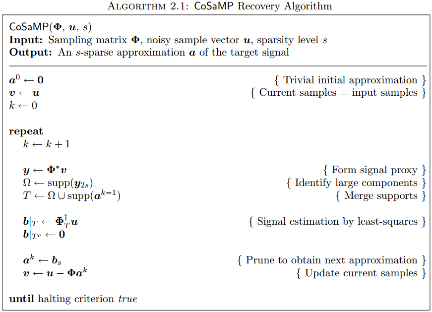
这个流程中的其它部分都可以看懂，就是那句“b|Tc←0”很不明白，“Tc”到底是指的什么呢？现在看来应该是T的补集(complementary set)，向量b的元素序号为全集，子集T对应的元素等于最小二乘解，补集对应的元素为零。

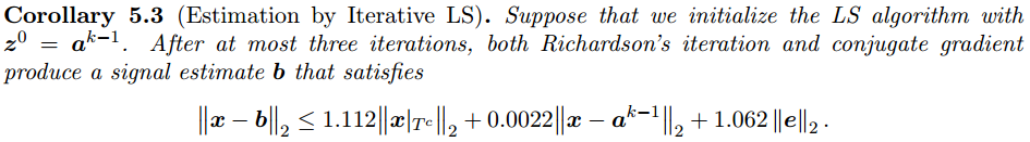
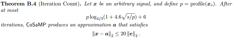
有关算法流程中的“注3”提到的迭代次数，在文献[2]中多处有提及，不过面向的问题不同，可以文献[2]中搜索“Iteration Count”，以下给出三处：

文献[8]的3.4节提到“设算法的迭代步长为K，候选集中最多有3K个原子，每次最多剔除K个原子，以保证支撑集中有2K个原子”，对这个观点我保留意见，我认为应该是“每次最多剔除2K个原子，以保证支撑集中有K个原子”。

参考文献：

[1]D. Needell, J.A. Tropp, CoSaMP: Iterative signal recovery from incomplete andinaccurate samples, ACM Technical Report 2008-01, California Institute ofTechnology, Pasadena, 2008.

(http://authors.library.caltech.edu/27169/)

[2]D. Needell, J.A. Tropp．CoSaMP: Iterative signal recoveryfrom incomplete and inaccurate samples.http://arxiv.org/pdf/0803.2392v2.pdf

[3] D. Needell, J.A. Tropp．CoSaMP：Iterativesignal recovery from incomplete and inaccurate samples[J]．Appliedand Computation Harmonic Analysis，2009，26：301-321.

(http://www.sciencedirect.com/science/article/pii/S1063520308000638)

[4]D.Needell, J.A. Tropp．CoSaMP: Iterative signal recoveryfrom incomplete and inaccurate samples[J]. Communications of theACM，2010，53(12)：93-100.

(http://dl.acm.org/citation.cfm?id=1859229)

[5]Li Zeng. CS_Reconstruction.http://www.pudn.com/downloads518/sourcecode/math/detail2151378.html

[6]wanghui.csmp. http://www.pudn.com/downloads252/sourcecode/others/detail1168584.html

[7]付自杰.cs_matlab. http://www.pudn.com/downloads641/sourcecode/math/detail2595379.html

[8]杨真真，杨震，孙林慧.信号压缩重构的正交匹配追踪类算法综述[J]. 信号处理，2013，29(4)：486-496.