Deeplearning学习之路_第四章（Self-Taught learning&deep networks）

最新推荐文章于 2018-10-26 13:48:30 发布

zCGr_GzGy

最新推荐文章于 2018-10-26 13:48:30 发布

阅读量1.7k

点赞数

分类专栏：机器学习 Deep Learning 文章标签： Deeplearning 机器学习神经网络

本文链接：https://blog.csdn.net/zCGr_GzGy/article/details/12311181

版权

机器学习同时被 2 个专栏收录

5 篇文章 0 订阅

订阅专栏

Deep Learning

5 篇文章 0 订阅

订阅专栏

一些笔记：

1）自我学习（Self—Taught learning）：

1.自我学习是一种学习特征的方法；

2.对于一些无标号（unlabeled）的样本{x_1，...，x_m}，可以用利用它们训练一个稀疏自编码器，得到了该编码器中权重参数，可以每一个输入x_i计算它的激活值a_i，用这些得到的激活值替换（replacement Representation）x_i或者与原值x_i级联（Concatenation Representation）得到一个新的样本集；

3.使用自我学习得到的新的样本集的表现，无论是替换还是级联都有可能是比原来的样本更好的特征描述。通常为了计算方便和减少代价，采用替换的情况比较多，而采用级联的效果可能会更好些；

4.无论初始样本是否是有标号的样本，我们都可以利用自我学习的方式学习除一些新的特征；

5.如果是带有标号的样本，再利用一些有监督学习的方式训练一些分类器（svm，softmax等），对于任意的测试样本都须先经过之前学习的稀疏自编码器得到隐层激活值构建新的特征送入训练好的分类器进行分类；

6.在训练稀疏自编码器之前可能需要对原数据进行一些预处理，而我们需要保存这些预处理使用的变换的参数以对接下来新样本使用相同的变化，比如PCA使用的矩阵U等等，否则如果对新的样本做相同方式的预处理但是可能使用的参数不同，比如PCA就可能使用不同的特征值矩阵U，最后导致新样本与原来的进入分类器的样本具有不同的分布；

7.自我学习的方法和半监督学习的方式都可以对部分不带类标的数据进行学习，而自我学习更为强大，它不需要带类标的数据和不带类标的数据来源于同一个分布，这个特性使得自我学习比半监督学习的适用更广；

2）深度网络（deep networks）：

1.微调(fine-tuned)是在自我学习的基础上利用，将分开训练的稀疏自编码器和分类器合成一个大的深度神经网络，并利用所有的带标签数据在现有的参数下，做一次整体优化；

2.隐层越多的神经网络具有更强大的表达能力，但是训练一个深度网络会有几方面需要解决的问题；

3.对于一个深度网络而言，带标签的数据不足的情况下，很容易导致过拟合；（所以运用deep network通常是处理大数据的情况）

4.深度网络的代价函数是一个高度非凸的函数，有许多局部极值点，直观上说，通常的梯度下降法（共轭梯度下降法、L-BFGS等）并不能很好的优化这个函数。因此预训练(Pre-Train)带来的好处可能在选取了不错的初始点，使得在微调（fine-tuned）的时候能够收敛到不错的极值点；

5.梯度弥散：在使用反向传播算法计算梯度的时候，从输出层到最初那几层的梯度值会急剧的减小，导致代价函数对于最初几层的权重的导数非常小，所以最初几层的权重在迭代的过程变化的非常缓慢，称为梯度的弥散。

6.与梯度弥散相关的问题在于在深度网络最后的几层神经元的个数足够多时，可能选取最后几层就已经可以单独对有标签的数据进行分类，这就导致了整个深度网路的分类性能可能和由最后几层决定的浅网络的性能类似；

7.逐层贪婪的训练方法，将已经训练好的k-1层的参数固定，单独训练第k层的参数，直到训练完整个网络，最后利用有标签的数据对网络进行微调；

Self-Taught learning&deep networks编程练习题：

matlab经验总结：

使用心得：

由于本次编程题目用到了之前几乎所有的主要函数，在编写的过程中没有遇到的什么问题。只是觉得在matlab报和维度相关的错误的时候可以通过在附近代码处显示矩阵的维度来发现问题。

实验代码：

1)Self-Taught learning

feedForwardAutoencoder.m

function [activation] = feedForwardAutoencoder(theta, hiddenSize, visibleSize, data)

% theta: trained weights from the autoencoder
% visibleSize: the number of input units (probably 64) 
% hiddenSize: the number of hidden units (probably 25) 
% data: Our matrix containing the training data as columns.  So, data(:,i) is the i-th training example. 
  
% We first convert theta to the (W1, W2, b1, b2) matrix/vector format, so that this 
% follows the notation convention of the lecture notes. 

W1 = reshape(theta(1:hiddenSize*visibleSize), hiddenSize, visibleSize);
b1 = theta(2*hiddenSize*visibleSize+1:2*hiddenSize*visibleSize+hiddenSize);

%% ---------- YOUR CODE HERE --------------------------------------
%  Instructions: Compute the activation of the hidden layer for the Sparse Autoencoder.
activation = sigmoid( bsxfun(@plus,W1*data ,b1));

%-------------------------------------------------------------------

end

%-------------------------------------------------------------------
% Here's an implementation of the sigmoid function, which you may find useful
% in your computation of the costs and the gradients.  This inputs a (row or
% column) vector (say (z1, z2, z3)) and returns (f(z1), f(z2), f(z3)). 

function sigm = sigmoid(x)
    sigm = 1 ./ (1 + exp(-x));
end

stlExercise.m

%% CS294A/CS294W Self-taught Learning Exercise

%  Instructions
%  ------------
% 
%  This file contains code that helps you get started on the
%  self-taught learning. You will need to complete code in feedForwardAutoencoder.m
%  You will also need to have implemented sparseAutoencoderCost.m and 
%  softmaxCost.m from previous exercises.
%
%% ======================================================================
%  STEP 0: Here we provide the relevant parameters values that will
%  allow your sparse autoencoder to get good filters; you do not need to 
%  change the parameters below.

inputSize  = 28 * 28;
numLabels  = 5;
hiddenSize = 200;
sparsityParam = 0.1; % desired average activation of the hidden units.
                     % (This was denoted by the Greek alphabet rho, which looks like a lower-case "p",
		             %  in the lecture notes). 
lambda = 3e-3;       % weight decay parameter       
beta = 3;            % weight of sparsity penalty term   
maxIter = 400;

%% ======================================================================
%  STEP 1: Load data from the MNIST database
%
%  This loads our training and test data from the MNIST database files.
%  We have sorted the data for you in this so that you will not have to
%  change it.

% Load MNIST database files
mnistData   = loadMNISTImages('mnist/train-images-idx3-ubyte');
mnistLabels = loadMNISTLabels('mnist/train-labels-idx1-ubyte');

% Set Unlabeled Set (All Images)

% Simulate a Labeled and Unlabeled set
labeledSet   = find(mnistLabels >= 0 & mnistLabels <= 4);
unlabeledSet = find(mnistLabels >= 5);

numTrain = round(numel(labeledSet)/2);
trainSet = labeledSet(1:numTrain);
testSet  = labeledSet(numTrain+1:end);

unlabeledData = mnistData(:, unlabeledSet);

trainData   = mnistData(:, trainSet);
trainLabels = mnistLabels(trainSet)' + 1; % Shift Labels to the Range 1-5

testData   = mnistData(:, testSet);
testLabels = mnistLabels(testSet)' + 1;   % Shift Labels to the Range 1-5

% Output Some Statistics
fprintf('# examples in unlabeled set: %d\n', size(unlabeledData, 2));
fprintf('# examples in supervised training set: %d\n\n', size(trainData, 2));
fprintf('# examples in supervised testing set: %d\n\n', size(testData, 2));

%% ======================================================================
%  STEP 2: Train the sparse autoencoder
%  This trains the sparse autoencoder on the unlabeled training
%  images. 

%  Randomly initialize the parameters
theta = initializeParameters(hiddenSize, inputSize);

%% ----------------- YOUR CODE HERE ----------------------
%  Find opttheta by running the sparse autoencoder on
%  unlabeledTrainingImages

opttheta = theta; 
%  Use minFunc to minimize the function
addpath minFunc/
options.Method = 'lbfgs'; % Here, we use L-BFGS to optimize our cost
                          % function. Generally, for minFunc to work, you
                          % need a function pointer with two outputs: the
                          % function value and the gradient. In our problem,
                          % sparseAutoencoderCost.m satisfies this.
options.maxIter = 400;	  % Maximum number of iterations of L-BFGS to run 
options.display = 'on';


[opttheta, cost] = minFunc( @(p) sparseAutoencoderCost(p, ...
                                   inputSize, hiddenSize, ...
                                   lambda, sparsityParam, ...
                                   beta, unlabeledData), ...
                              theta, options);








%% -----------------------------------------------------
                          
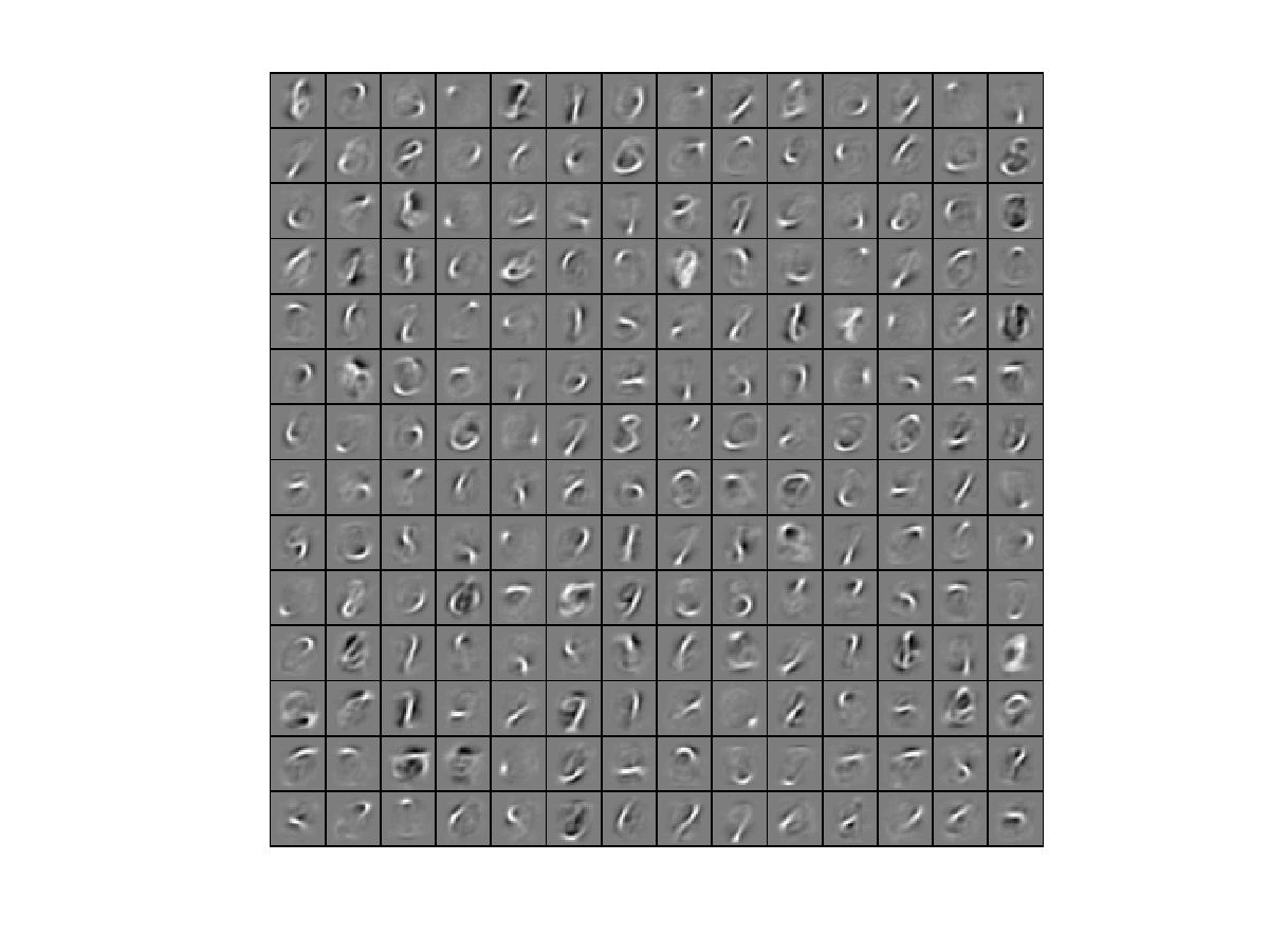
% Visualize weights
W1 = reshape(opttheta(1:hiddenSize * inputSize), hiddenSize, inputSize);
display_network(W1');

%%======================================================================
%% STEP 3: Extract Features from the Supervised Dataset
%  
%  You need to complete the code in feedForwardAutoencoder.m so that the 
%  following command will extract features from the data.

trainFeatures = feedForwardAutoencoder(opttheta, hiddenSize, inputSize, ...
                                       trainData);

testFeatures = feedForwardAutoencoder(opttheta, hiddenSize, inputSize, ...
                                       testData);

%%======================================================================
%% STEP 4: Train the softmax classifier

softmaxModel = struct;  
%% ----------------- YOUR CODE HERE ----------------------
%  Use softmaxTrain.m from the previous exercise to train a multi-class
%  classifier. 

%  Use lambda = 1e-4 for the weight regularization for softmax

% You need to compute softmaxModel using softmaxTrain on trainFeatures and
% trainLabels
options.maxIter = 100;
lambda = 1e-4;
inputSize = size(trainFeatures,1);
softmaxModel = softmaxTrain(inputSize, numLabels, lambda, ...
                            trainFeatures, trainLabels, options);








%% -----------------------------------------------------


%%======================================================================
%% STEP 5: Testing 

%% ----------------- YOUR CODE HERE ----------------------
% Compute Predictions on the test set (testFeatures) using softmaxPredict
% and softmaxModel

inputData = testFeatures;

% You will have to implement softmaxPredict in softmaxPredict.m
[pred] = softmaxPredict(softmaxModel, inputData);

acc = mean(testLabels(:) == pred(:));
fprintf('Accuracy: %0.3f%%\n', acc * 100);














%% -----------------------------------------------------

% Classification Score
fprintf('Test Accuracy: %f%%\n', 100*mean(pred(:) == testLabels(:)));

% (note that we shift the labels by 1, so that digit 0 now corresponds to
%  label 1)
%
% Accuracy is the proportion of correctly classified images
% The results for our implementation was:
%
% Accuracy: 98.3%
%
%

运行结果如下：

首先是将稀疏自编码器的权重可视化结果：

随后是分类结果：

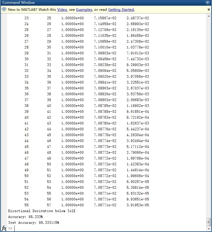
5分类问题，正确率98.33%,达到了题目要求的98%

该练习题详见：http://deeplearning.stanford.edu/wiki/index.php/Exercise:Self-Taught_Learning

2）deep networks

stackedAECost.m

function [ cost, grad ] = stackedAECost(theta, inputSize, hiddenSize, ...
                                              numClasses, netconfig, ...
                                              lambda, data, labels)
                                         
% stackedAECost: Takes a trained softmaxTheta and a training data set with labels,
% and returns cost and gradient using a stacked autoencoder model. Used for
% finetuning.
                                         
% theta: trained weights from the autoencoder
% visibleSize: the number of input units
% hiddenSize:  the number of hidden units *at the 2nd layer*
% numClasses:  the number of categories
% netconfig:   the network configuration of the stack
% lambda:      the weight regularization penalty
% data: Our matrix containing the training data as columns.  So, data(:,i) is the i-th training example. 
% labels: A vector containing labels, where labels(i) is the label for the
% i-th training example


%% Unroll softmaxTheta parameter

% We first extract the part which compute the softmax gradient
softmaxTheta = reshape(theta(1:hiddenSize*numClasses), numClasses, hiddenSize);

% Extract out the "stack"
stack = params2stack(theta(hiddenSize*numClasses+1:end), netconfig);

% You will need to compute the following gradients
softmaxThetaGrad = zeros(size(softmaxTheta));
stackgrad = cell(size(stack));
hiddenLayers = numel(stack);
for d = 1:hiddenLayers
    stackgrad{d}.w = zeros(size(stack{d}.w));
    stackgrad{d}.b = zeros(size(stack{d}.b));
%     fprintf('%dth Layer ,w = %d x %d , b = %d x %d\n',d,size(stack{d}.w,1),size(stack{d}.w,2),size(stack{d}.b,1),size(stack{d}.b,2));
end

cost = 0; % You need to compute this

% You might find these variables useful
M = size(data, 2);
groundTruth = full(sparse(labels, 1:M, 1));


%% --------------------------- YOUR CODE HERE -----------------------------
%  Instructions: Compute the cost function and gradient vector for 
%                the stacked autoencoder.
%
%                You are given a stack variable which is a cell-array of
%                the weights and biases for every layer. In particular, you
%                can refer to the weights of Layer d, using stack{d}.w and
%                the biases using stack{d}.b . To get the total number of
%                layers, you can use numel(stack).
%
%                The last layer of the network is connected to the softmax
%                classification layer, softmaxTheta.
%
%                You should compute the gradients for the softmaxTheta,
%                storing that in softmaxThetaGrad. Similarly, you should
%                compute the gradients for each layer in the stack, storing
%                the gradients in stackgrad{d}.w and stackgrad{d}.b
%                Note that the size of the matrices in stackgrad should
%                match exactly that of the size of the matrices in stack.
%


% initialize for act and delta
act = zeros(hiddenLayers*hiddenSize + numClasses, M);
delta = zeros(hiddenLayers*hiddenSize + numClasses, M);

%forwardpropogation
act(1:hiddenSize,:) = sigmoid(bsxfun(@plus, stack{1}.w*data, stack{1}.b));  
for d = 2:hiddenLayers
    act((d-1)*hiddenSize+1:d*hiddenSize,:) = sigmoid(bsxfun(@plus, stack{d}.w * act((d-2)*hiddenSize+1:(d-1)*hiddenSize,:), stack{d}.b));
end
Me = softmaxTheta * act((hiddenLayers-1)*hiddenSize+1:hiddenLayers*hiddenSize,:);
Me = exp(bsxfun(@minus ,Me ,max(Me ,[] ,1)));
Me = bsxfun(@rdivide ,Me ,sum(Me));
act(d*hiddenSize+1:end,:) = Me;

%backpropogation
% Me = exp(bsxfun(@minus ,Me ,max(Me ,[] ,1)));
% Me = bsxfun(@rdivide ,Me ,sum(Me));
delta(hiddenLayers*hiddenSize+1:end,:) = -1/M*(groundTruth - Me);
delta( (hiddenLayers - 1) * hiddenSize + 1 : hiddenLayers * hiddenSize,: ) = softmaxTheta'* delta(hiddenLayers*hiddenSize+1:end,:)...
    .* (act( (hiddenLayers - 1) * hiddenSize + 1 : hiddenLayers * hiddenSize,:).*( 1 - act( (hiddenLayers - 1) * hiddenSize + 1 :...
    hiddenLayers * hiddenSize,:))) ;
for d = 2 : hiddenLayers
    delta( (hiddenLayers - d)* hiddenSize + 1 : (hiddenLayers - d + 1)* hiddenSize,:) = stack{hiddenLayers - d + 2}.w'* delta( (hiddenLayers - d + 1)...
        * hiddenSize + 1 : (hiddenLayers - d + 2)* hiddenSize,:) .* (act( (hiddenLayers - d)* hiddenSize + 1 : (hiddenLayers - d + 1)* hiddenSize,:).*( 1 - ...
        act( (hiddenLayers - d)* hiddenSize + 1 : (hiddenLayers - d + 1)* hiddenSize,:)));
end
% disp(size(Me));
% disp(size(act(hiddenLayers*hiddenSize+1:end,:)'));
% disp(size(softmaxTheta));
softmaxThetaGrad = delta(hiddenLayers*hiddenSize+1:end,:) * act( (hiddenLayers-1)*hiddenSize+1:hiddenLayers*hiddenSize,:)' + lambda * softmaxTheta;
stackgrad{1}.w = delta(1:hiddenSize,:)*data';
stackgrad{1}.b = sum(delta(1:hiddenSize,:)')';
for d = 2:hiddenLayers
    stackgrad{d}.w = delta((d-1)*hiddenSize+1:d*hiddenSize,:)*act((d-2)*hiddenSize+1:(d-1)*hiddenSize,:)';
    stackgrad{d}.b = sum(delta((d-1)*hiddenSize+1:d*hiddenSize,:)')';
end
cost = -1/M*sum(sum(groundTruth.*log(Me))) + lambda/2 * norm(softmaxTheta,'fro')^2;











% -------------------------------------------------------------------------

%% Roll gradient vector
grad = [softmaxThetaGrad(:) ; stack2params(stackgrad)];

end


% You might find this useful
function sigm = sigmoid(x)
    sigm = 1 ./ (1 + exp(-x));
end

stackedAEPredict.m

function [pred] = stackedAEPredict(theta, inputSize, hiddenSize, numClasses, netconfig, data)
                                         
% stackedAEPredict: Takes a trained theta and a test data set,
% and returns the predicted labels for each example.
                                         
% theta: trained weights from the autoencoder
% visibleSize: the number of input units
% hiddenSize:  the number of hidden units *at the 2nd layer*
% numClasses:  the number of categories
% data: Our matrix containing the training data as columns.  So, data(:,i) is the i-th training example. 

% Your code should produce the prediction matrix 
% pred, where pred(i) is argmax_c P(y(c) | x(i)).
 
%% Unroll theta parameter

% We first extract the part which compute the softmax gradient
softmaxTheta = reshape(theta(1:hiddenSize*numClasses), numClasses, hiddenSize);

% Extract out the "stack"
stack = params2stack(theta(hiddenSize*numClasses+1:end), netconfig);

%% ---------- YOUR CODE HERE --------------------------------------
%  Instructions: Compute pred using theta assuming that the labels start 
%                from 1.
hiddenLayers = numel(stack);
M = size(data,2);
pred = zeros(1, M);
act = zeros(hiddenLayers*hiddenSize, M);

%forwardpropogation
act(1:hiddenSize,:) = sigmoid(bsxfun(@plus, stack{1}.w*data, stack{1}.b));  
for d = 2:hiddenLayers
    act((d-1)*hiddenSize+1:d*hiddenSize,:) = sigmoid(bsxfun(@plus, stack{d}.w * act((d-2)*hiddenSize+1:(d-1)*hiddenSize,:), stack{d}.b));
end
Me = softmaxTheta * act((hiddenLayers-1)*hiddenSize+1:hiddenLayers*hiddenSize,:);
[~,pred] = max(Me ,[] ,1);









% -----------------------------------------------------------

end


% You might find this useful
function sigm = sigmoid(x)
    sigm = 1 ./ (1 + exp(-x));
end

stackedAEExercise.m

function [pred] = stackedAEPredict(theta, inputSize, hiddenSize, numClasses, netconfig, data)
                                         
% stackedAEPredict: Takes a trained theta and a test data set,
% and returns the predicted labels for each example.
                                         
% theta: trained weights from the autoencoder
% visibleSize: the number of input units
% hiddenSize:  the number of hidden units *at the 2nd layer*
% numClasses:  the number of categories
% data: Our matrix containing the training data as columns.  So, data(:,i) is the i-th training example. 

% Your code should produce the prediction matrix 
% pred, where pred(i) is argmax_c P(y(c) | x(i)).
 
%% Unroll theta parameter

% We first extract the part which compute the softmax gradient
softmaxTheta = reshape(theta(1:hiddenSize*numClasses), numClasses, hiddenSize);

% Extract out the "stack"
stack = params2stack(theta(hiddenSize*numClasses+1:end), netconfig);

%% ---------- YOUR CODE HERE --------------------------------------
%  Instructions: Compute pred using theta assuming that the labels start 
%                from 1.
hiddenLayers = numel(stack);
M = size(data,2);
pred = zeros(1, M);
act = zeros(hiddenLayers*hiddenSize, M);

%forwardpropogation
act(1:hiddenSize,:) = sigmoid(bsxfun(@plus, stack{1}.w*data, stack{1}.b));  
for d = 2:hiddenLayers
    act((d-1)*hiddenSize+1:d*hiddenSize,:) = sigmoid(bsxfun(@plus, stack{d}.w * act((d-2)*hiddenSize+1:(d-1)*hiddenSize,:), stack{d}.b));
end
Me = softmaxTheta * act((hiddenLayers-1)*hiddenSize+1:hiddenLayers*hiddenSize,:);
[~,pred] = max(Me ,[] ,1);









% -----------------------------------------------------------

end


% You might find this useful
function sigm = sigmoid(x)
    sigm = 1 ./ (1 + exp(-x));
end

运行结果如下：