Deeplearning学习之路_第二章（Vectorization&PCA）

一些笔记：

1）Vectorization

1.对于matlab编程，将数据向量化后，利用matlab的函数提供的强大的矩阵处理功能对数据进行处理将比写C—style的显示循环处理数据的效率要高很多，所以要在不断的练习中客服使用显示循环的习惯。

2）PCA

1.对于输入数据的特征之间可能存在高度相关的数据（比如图像），这种数据一般都称为冗余数据。面对这种数据时，我们的第一反应就是如何提取数据中有用的信息，这对我们带来的好处将是数据规模的减小，使得我们的代码运行速度得到提升；

2.PCA算法便是这样一种算法，它可以在保留原有数据绝大部分信息的同时对数据进行比较大幅度的降维，是一种很好的降维算法；

3.使用PCA算法需要对数据进行预处理，也就是对数据进行均值归整化；由于PCA算法对于输入数据具有伸缩不变性，即：将每个数据都扩大相同的倍数，输出的特征向量都不变；

4.对图像数据进行去均值归整化的时候，可以用一种近似处理的办法，用每一个像素点的值减去该图像所有点的均值即可；

5.对数据做完预处理过后，数据的协方差矩阵sigma=1/m*(sum_{1}_{m}x_i*Transpose(x_i))，如果用X表示所有数据的话（每一列是一个样本）那么sigma = X*Transpose(X)/m

6.对sigma进行SVD分解，求出sigma的特征向量矩阵U和特征值矩阵S，我们记xRot = Transpose(U)*X;S矩阵的对角线上数值从左上到右下按照从大到小排列；

7.将xRot保留前K个分量，后面的分量取成0构成了PCA算法结果xHat，而我们只取xHat的前K个分量（非零）放入我们的程序，进行我们需要的运算；

8.关于K的取法。用前K个特征值之和除总的特征值之后作为方差（variance）保留百分比，而使得该比率大于某个分位点的最小的K值，该分位点通常取90%~98%之间，图像数据通常取99%；

9.理论上，图像的任何一个部分的统计性质都应该和其他部分相同，图像的这种特性被称作平稳性。（Stationarity）

3）白化（Sphering）

1.白化的目的同样在于降低数据的冗余性；

2.白化的目的：使得特征之间的相关性降低；使得所有特征的方差相同；

3.在PCA中，xRot_i的各个分量之间已经不相关了（因为xRot被一组单位正交基，即sigma的特征向量表示），所以为了使得输入特征的协方差矩阵sigma=I单位阵，可以做变换： x_PCAWhite,i = xRot_i/sqrt( lambda_i ) ，lambda_i表示第i个特征值, xRot_i/表示xRot的第i个分量。

4.如果需要降维的话，也可以去x_PCAWhite的前K个分量，K取法同前；

5.ZCA白化：与PCA不同的是，ZCA白化不做降维处理；

6.对于任意的单位正交阵R。R*xPCAWhite具有单位协方差，但是U为sigma的特征向量时，使得xZCA  = U*xPCAWhite 最接近原数据。

7.正则化：在PCA白化的过程中，可能会由于本征值过小而出现在分母导致数据上溢（出现大数值或者不稳定），我们通常给lambda加上一个很小的数epsilon。对于图像而言，正则化是的图像更加平滑。

Vectorization&PCA编程练习题：

matlab经验总结：

函数类：

1,使用bsxfun的效率比repmat 的效率更高，repmat是显式的复制，当然带来内存的消耗。而bsxfun是虚拟的复制，实际上通过for来实现,但bsxfun不会有使用matlab的for所带来额外时间；参加bsxfun浅谈

2.cumsum函数求得前n项部分和，比如A=[1,2,3,4] 	cumsum（A）=[1,3,6,10]

使用心得：

在数据量比较大的时候比较容易out of memory，做开始在32位机器上做Mnist的时候总是爆内存，后来查了很多方法，感觉最有效果的还是换成64位的系统。另外在使用变量的时候要先申明变量初始化，形成好的编码习惯

实验代码（matlab）：

1.Vectorization

由于上一节练习神经网络的时候已经将神经网络前向传播和方向传播中的显示循环向量化了，在此就不贴出来了。所以这一节剩下的任务就是改一下上次的参数而已：

Mnist.m：

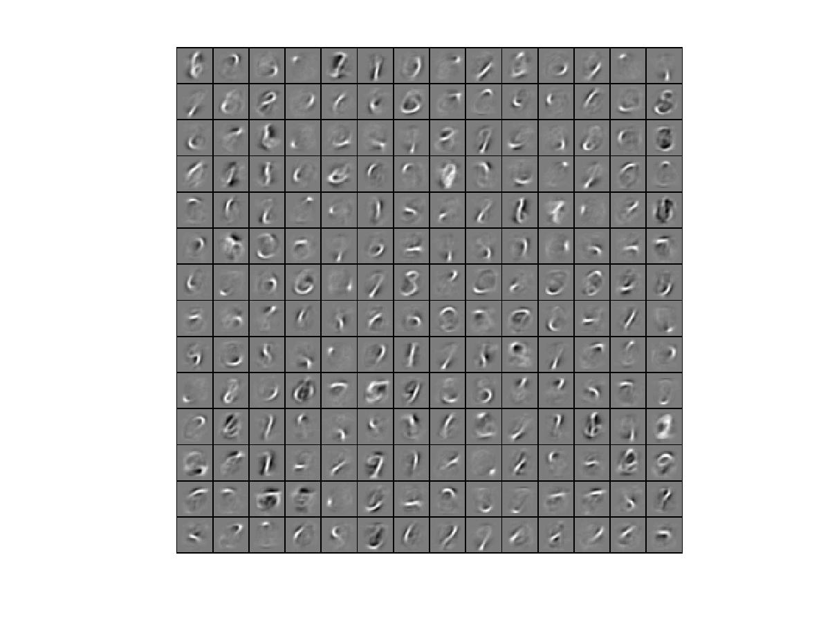
clear all;
IMAGES = loadMNISTImages('train-images-idx3-ubyte');

patchsize = 28;  % we'll use 8x8 patches 
numpatches = 10000;

% Initialize patches with zeros.  Your code will fill in this matrix--one
% column per patch, 10000 columns. 
% patches = zeros(patchsize*patchsize, numpatches);

%in order to speed up the code , an effective way is to decrease the times 
%copying big image matrix. So I decide to ensure how many patches to get from 
%each image before copying them.

patches = IMAGES(:,1:numpatches);
% % patches = patch2vec(Images);
clear IMAGES;

visibleSize = 28*28;
hiddenSize = 196;
sparsityParam = 0.1;
lambda = 3*10^(-3);
beta = 3;

display_network(patches(:,randi(size(patches,2),200,1)),8);


%  Obtain random parameters theta
theta = initializeParameters(hiddenSize, visibleSize);

%%======================================================================
%% STEP 2: Implement sparseAutoencoderCost
%
%  You can implement all of the components (squared error cost, weight decay term,
%  sparsity penalty) in the cost function at once, but it may be easier to do 
%  it step-by-step and run gradient checking (see STEP 3) after each step.  We 
%  suggest implementing the sparseAutoencoderCost function using the following steps:
%
%  (a) Implement forward propagation in your neural network, and implement the 
%      squared error term of the cost function.  Implement backpropagation to 
%      compute the derivatives.   Then (using lambda=beta=0), run Gradient Checking 
%      to verify that the calculations corresponding to the squared error cost 
%      term are correct.
%
%  (b) Add in the weight decay term (in both the cost function and the derivative
%      calculations), then re-run Gradient Checking to verify correctness. 
%
%  (c) Add in the sparsity penalty term, then re-run Gradient Checking to 
%      verify correctness.
%
%  Feel free to change the training settings when debugging your
%  code.  (For example, reducing the training set size or 
%  number of hidden units may make your code run faster; and setting beta 
%  and/or lambda to zero may be helpful for debugging.)  However, in your 
%  final submission of the visualized weights, please use parameters we 
%  gave in Step 0 above.

[cost, grad] = sparseAutoencoderCost(theta, visibleSize, hiddenSize, lambda, ...
                                     sparsityParam, beta, patches);

%%======================================================================
% %% STEP 3: Gradient Checking
% %
% % Hint: If you are debugging your code, performing gradient checking on smaller models 
% % and smaller training sets (e.g., using only 10 training examples and 1-2 hidden 
% % units) may speed things up.
% 
% % First, lets make sure your numerical gradient computation is correct for a
% % simple function.  After you have implemented computeNumericalGradient.m,
% % run the following: 
% checkNumericalGradient();
% 
% % Now we can use it to check your cost function and derivative calculations
% % for the sparse autoencoder.  
% numgrad = computeNumericalGradient( @(x) sparseAutoencoderCost(x, visibleSize, ...
%                                                   hiddenSize, lambda, ...
%                                                   sparsityParam, beta, ...
%                                                   patches), theta);
% 
% % Use this to visually compare the gradients side by side
% disp([numgrad grad]); 
% 
% % Compare numerically computed gradients with the ones obtained from backpropagation
% diff = norm(numgrad-grad)/norm(numgrad+grad);
% disp(diff); % Should be small. In our implementation, these values are
%             % usually less than 1e-9.
% 
%             % When you got this working, Congratulations!!! 

%%======================================================================
%% STEP 4: After verifying that your implementation of
%  sparseAutoencoderCost is correct, You can start training your sparse
%  autoencoder with minFunc (L-BFGS).

%  Randomly initialize the parameters
theta = initializeParameters(hiddenSize, visibleSize);

%  Use minFunc to minimize the function
addpath minFunc/
options.Method = 'lbfgs'; % Here, we use L-BFGS to optimize our cost
                          % function. Generally, for minFunc to work, you
                          % need a function pointer with two outputs: the
                          % function value and the gradient. In our problem,
                          % sparseAutoencoderCost.m satisfies this.
options.maxIter = 400;	  % Maximum number of iterations of L-BFGS to run 
options.display = 'on';


[opttheta, cost] = minFunc( @(p) sparseAutoencoderCost(p, ...
                                   visibleSize, hiddenSize, ...
                                   lambda, sparsityParam, ...
                                   beta, patches), ...
                              theta, options);

%%======================================================================
%% STEP 5: Visualization 

W1 = reshape(opttheta(1:hiddenSize*visibleSize), hiddenSize, visibleSize);
display_network(W1', 12); 

print -djpeg weights.jpg   % save the visualization to a file 

实验结果如下：

2.PCA

这一次的练习工作量很少，代码如下：

pca_2d.m

close all

%%================================================================
%% Step 0: Load data
%  We have provided the code to load data from pcaData.txt into x.
%  x is a 2 * 45 matrix, where the kth column x(:,k) corresponds to
%  the kth data point.Here we provide the code to load natural image data into x.
%  You do not need to change the code below.

x = load('pcaData.txt','-ascii');
figure(1);
scatter(x(1, :), x(2, :));
title('Raw data');


%%================================================================
%% Step 1a: Implement PCA to obtain U 
%  Implement PCA to obtain the rotation matrix U, which is the eigenbasis
%  sigma. 

% -------------------- YOUR CODE HERE -------------------- 
u = zeros(size(x, 1)); % You need to compute this
sigma = x*x'/size(x,2);
[u s v] = svd(sigma);



% -------------------------------------------------------- 
hold on
plot([0 u(1,1)], [0 u(2,1)]);
plot([0 u(1,2)], [0 u(2,2)]);
scatter(x(1, :), x(2, :));
hold off

%%================================================================
%% Step 1b: Compute xRot, the projection on to the eigenbasis
%  Now, compute xRot by projecting the data on to the basis defined
%  by U. Visualize the points by performing a scatter plot.

% -------------------- YOUR CODE HERE -------------------- 
xRot = zeros(size(x)); % You need to compute this
xRot = u'*x;


% -------------------------------------------------------- 

% Visualise the covariance matrix. You should see a line across the
% diagonal against a blue background.
figure(2);
scatter(xRot(1, :), xRot(2, :));
title('xRot');

%%================================================================
%% Step 2: Reduce the number of dimensions from 2 to 1. 
%  Compute xRot again (this time projecting to 1 dimension).
%  Then, compute xHat by projecting the xRot back onto the original axes 
%  to see the effect of dimension reduction

% -------------------- YOUR CODE HERE -------------------- 
k = 1; % Use k = 1 and project the data onto the first eigenbasis
xHat = zeros(size(x)); % You need to compute this
xHat = u(:,1:k)'*x;
xHat = u*[xHat;zeros(size(x,1)-k,size(x,2))];


% -------------------------------------------------------- 
figure(3);
scatter(xHat(1, :), xHat(2, :));
title('xHat');


%%================================================================
%% Step 3: PCA Whitening
%  Complute xPCAWhite and plot the results.

epsilon = 1e-5;
% -------------------- YOUR CODE HERE -------------------- 
xPCAWhite = zeros(size(x)); % You need to compute this
xPCAWhite = diag(diag(1./sqrt(s+epsilon)))*xRot;


% -------------------------------------------------------- 
figure(4);
scatter(xPCAWhite(1, :), xPCAWhite(2, :));
title('xPCAWhite');

%%================================================================
%% Step 3: ZCA Whitening
%  Complute xZCAWhite and plot the results.

% -------------------- YOUR CODE HERE -------------------- 
xZCAWhite = zeros(size(x)); % You need to compute this
xZCAWhite = u*xPCAWhite;

% -------------------------------------------------------- 
figure(5);
scatter(xZCAWhite(1, :), xZCAWhite(2, :));
title('xZCAWhite');

%% Congratulations! When you have reached this point, you are done!
%  You can now move onto the next PCA exercise. :)

实验结果符合题目要求，题目要求见：Exercise：PCA_2D

pca_gen.m

%%================================================================
%% Step 0a: Load data
%  Here we provide the code to load natural image data into x.
%  x will be a 144 * 10000 matrix, where the kth column x(:, k) corresponds to
%  the raw image data from the kth 12x12 image patch sampled.
%  You do not need to change the code below.

x = sampleIMAGESRAW();
figure('name','Raw images');
randsel = randi(size(x,2),200,1); % A random selection of samples for visualization
display_network(x(:,randsel));

%%================================================================
%% Step 0b: Zero-mean the data (by row)
%  You can make use of the mean and repmat/bsxfun functions.

% -------------------- YOUR CODE HERE -------------------- 
x = bsxfun(@minus, x,mean(x));
%%================================================================
%% Step 1a: Implement PCA to obtain xRot
%  Implement PCA to obtain xRot, the matrix in which the data is expressed
%  with respect to the eigenbasis of sigma, which is the matrix U.


% -------------------- YOUR CODE HERE -------------------- 
xRot = zeros(size(x)); % You need to compute this
sigma = x*x'/size(x,2);
[U S V] = svd(sigma);
xRot = U'*x;

%%================================================================
%% Step 1b: Check your implementation of PCA
%  The covariance matrix for the data expressed with respect to the basis U
%  should be a diagonal matrix with non-zero entries only along the main
%  diagonal. We will verify this here.
%  Write code to compute the covariance matrix, covar. 
%  When visualised as an image, you should see a straight line across the
%  diagonal (non-zero entries) against a blue background (zero entries).

% -------------------- YOUR CODE HERE -------------------- 
covar = zeros(size(x, 1)); % You need to compute this
covar = xRot*xRot'/size(xRot,2);
% Visualise the covariance matrix. You should see a line across the
% diagonal against a blue background.
figure('name','Visualisation of covariance matrix');
imagesc(covar);

%%================================================================
%% Step 2: Find k, the number of components to retain
%  Write code to determine k, the number of components to retain in order
%  to retain at least 99% of the variance.

% -------------------- YOUR CODE HERE -------------------- 
k = 0; % Set k accordingly
M = 0.99*sum(diag(S));
k = find(cumsum(diag(S)) > M, 1 );
%%================================================================
%% Step 3: Implement PCA with dimension reduction
%  Now that you have found k, you can reduce the dimension of the data by
%  discarding the remaining dimensions. In this way, you can represent the
%  data in k dimensions instead of the original 144, which will save you
%  computational time when running learning algorithms on the reduced
%  representation.
% 
%  Following the dimension reduction, invert the PCA transformation to produce 
%  the matrix xHat, the dimension-reduced data with respect to the original basis.
%  Visualise the data and compare it to the raw data. You will observe that
%  there is little loss due to throwing away the principal components that
%  correspond to dimensions with low variation.

% -------------------- YOUR CODE HERE -------------------- 
xHat = zeros(size(x));  % You need to compute this
xHat = U(:,1:k)'*x;
xHat = U*[xHat;zeros(size(x,1)-k,size(x,2))];


% Visualise the data, and compare it to the raw data
% You should observe that the raw and processed data are of comparable quality.
% For comparison, you may wish to generate a PCA reduced image which
% retains only 90% of the variance.

figure('name',['PCA processed images ',sprintf('(%d / %d dimensions)', k, size(x, 1)),'']);
display_network(xHat(:,randsel));
figure('name','Raw images');
display_network(x(:,randsel));

%%================================================================
%% Step 4a: Implement PCA with whitening and regularisation
%  Implement PCA with whitening and regularisation to produce the matrix
%  xPCAWhite. 

epsilon = 0.1;
xPCAWhite = zeros(size(x));

% -------------------- YOUR CODE HERE -------------------- 
xPCAWhite = diag(1./sqrt(diag(S)+epsilon))*xRot;
%%================================================================
%% Step 4b: Check your implementation of PCA whitening 
%  Check your implementation of PCA whitening with and without regularisation. 
%  PCA whitening without regularisation results a covariance matrix 
%  that is equal to the identity matrix. PCA whitening with regularisation
%  results in a covariance matrix with diagonal entries starting close to 
%  1 and gradually becoming smaller. We will verify these properties here.
%  Write code to compute the covariance matrix, covar. 
%
%  Without regularisation (set epsilon to 0 or close to 0), 
%  when visualised as an image, you should see a red line across the
%  diagonal (one entries) against a blue background (zero entries).
%  With regularisation, you should see a red line that slowly turns
%  blue across the diagonal, corresponding to the one entries slowly
%  becoming smaller.

% -------------------- YOUR CODE HERE -------------------- 
covar = xPCAWhite*xPCAWhite'/size(xPCAWhite,2);
% Visualise the covariance matrix. You should see a red line across the
% diagonal against a blue background.
figure('name','Visualisation of covariance matrix');
imagesc(covar);

%%================================================================
%% Step 5: Implement ZCA whitening
%  Now implement ZCA whitening to produce the matrix xZCAWhite. 
%  Visualise the data and compare it to the raw data. You should observe
%  that whitening results in, among other things, enhanced edges.

xZCAWhite = zeros(size(x));

% -------------------- YOUR CODE HERE -------------------- 
xZCAWhite = U*xPCAWhite;
% Visualise the data, and compare it to the raw data.
% You should observe that the whitened images have enhanced edges.
figure('name','ZCA whitened images');
display_network(xZCAWhite(:,randsel));
figure('name','Raw images');
display_network(x(:,randsel));

实验结果符合题目要求，题目要求见：Exercise：PCA&Whiting