pandas绘图

pandas绘图显示 : plt.show()

保存到本地 : plt.savefig(‘image.png’)

%matplotlib inline

• 1

import pandas as pd
import matplotlib.pyplot as plt

• 1
• 2

present = pd.read_table('data.txt', sep=' ')

• 1

present.shape

• 1

(63, 3)

present.columns

• 1

Index([u’year’, u’boys’, u’girls’], dtype=’object’) 可以看到这个数据集共有63条记录，共有三个字段：Year，boys，girls。为了简化计算将year作为索引

present_year = present.set_index('year')

• 1

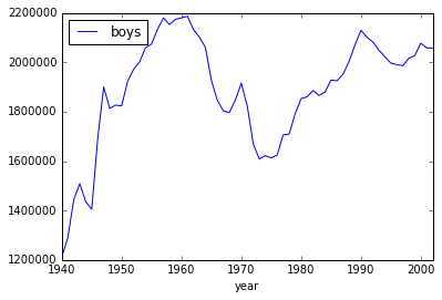
plot是画图的最主要方法，Series和DataFrame都有plot方法。 我们可以这样看一下男生出生比例的趋势图：

present_year['boys'].plot()
plt.legend(loc='best')

• 1
• 2

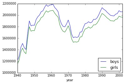
 这是Series上的plot方法，通过DataFrame的plot方法，你可以将男生和女生出生数量的趋势图画在一起。

present_year.plot()       #has index,column

• 1


present_year.girls.plot(color='g')
present_year.boys.plot(color='b')
plt.legend(loc='best')

• 1
• 2
• 3

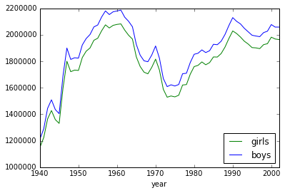 可以看到DataFrame提供plot方法与在多个Series调用多次plot方法的效果是一致。

present_year[:10].plot(kind='bar')

• 1

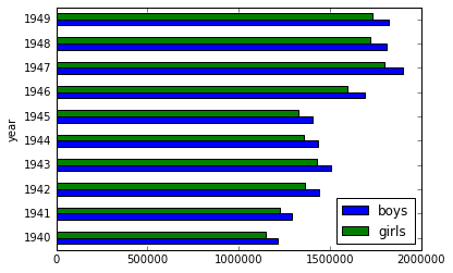
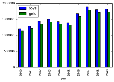 plot默认生成是曲线图，你可以通过kind参数生成其他的图形，可选的值为：line, bar, barh, kde, density, scatter。

present_year[:10].plot(kind='barh')

• 1

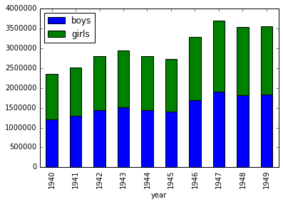
 如果你需要累积的柱状图，则只需要指定stacked=True。

present_year[:10].plot(kind='bar', stacked=True)

• 1

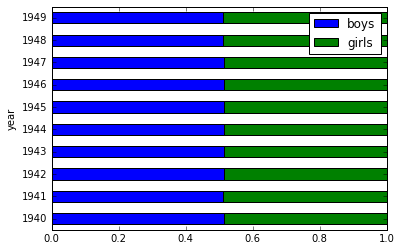
 制作相对的累积柱状图，需要一点小技巧。 首先需要计算每一行的汇总值，可以在DataFrame上直接调用sum方法，参数为1，表示计算行的汇总。默认为0，表示计算列的汇总。

present_year.sum(1)[:5]

• 1

year 1940 2360399 1941 2513427 1942 2808996 1943 2936860 1944 2794800 dtype: int64 有了每一行的汇总值之后，再用每个元素除以对应行的汇总值就可以得出需要的数据。这里可以使用DataFrame的div函数，同样要指定axis的值为0。

present_year.div(present_year.sum(1),axis=0)[:10].plot(kind='barh', stacked=True)

• 1

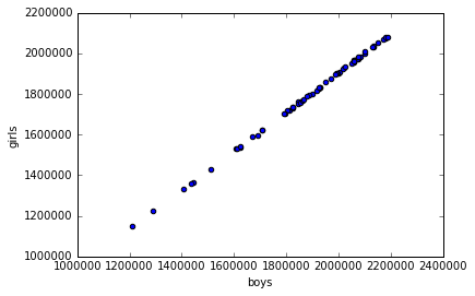
 散点图和相关 plot也可以画出散点图。使用kind=’scatter’, x和y指定x轴和y轴使用的字段。

present_year.plot(x='boys', y='girls', kind='scatter')

• 1

 我们再来载入一下鸢尾花数据。

iris = pd.read_csv('iris.csv')
iris.head(5)

SepalLength SepalWidth PetalLength PetalWidth Name 0 5.1 3.5 1.4 0.2 Iris-setosa 1 4.9 3.0 1.4 0.2 Iris-setosa 2 4.7 3.2 1.3 0.2 Iris-setosa 3 4.6 3.1 1.5 0.2 Iris-setosa 4 5.0 3.6 1.4 0.2 Iris-setosa iris.corr() 1   SepalLength SepalWidth PetalLength PetalWidth SepalLength 1.000000 -0.109369 0.871754 0.817954 SepalWidth -0.109369 1.000000 -0.420516 -0.356544 PetalLength 0.871754 -0.420516 1.000000 0.962757 PetalWidth 0.817954 -0.356544 0.962757 1.000000 from pandas.tools.plotting import scatter_matrix scatter_matrix(iris, alpha=0.2, figsize=(6, 6), diagonal='kde') 箱图 DataFrame提供了boxplot方法可以用来画箱图。 iris.boxplot()   iris.boxplot(by='Name', figsize=(8, 8)) 1 直方图和概率密度分布 iris.ix[:,:-1].hist() iris.plot(kind='kde') 多变量的可视化 Radviz from pandas.tools.plotting import radviz radviz(iris, 'Name') from pandas.tools.plotting import andrews_curves andrews_curves(iris, 'Name') Parallel Coordinates from pandas.tools.plotting import parallel_coordinates parallel_coordinates(iris, 'Name')