利用TensorFlow和Keras进行Btcoin价格预测

https://mp.weixin.qq.com/s?__biz=MzU1NDA4NjU2MA%3D%3D&mid=2247487867&idx=4&sn=97e9a472eb2fea3c8194772be021a45c&chksm=fbe9a8b4cc9e21a210d71a18cebbb62d4e737040f6e1fe2709974a8a65adbc494df5bd9f08ed&scene=0&key=ceb62083117db9ae54b9d2fa5a2020f33f99a74fd6a92816085ea7805587812c51f3ea7932b54f52c10b6d844af3bf1477fb3b84cde2b99cee26f2b25b107c5836e3683064db3dab390536477bb507fc&ascene=0&uin=MjEzMTAwMzgyNQ%3D%3D&devicetype=iMac+MacBookAir7%2C1+OSX+OSX+10.12.6+build%2816G29%29&version=12020810&nettype=WIFI&lang=zh_CN&fontS

电子加密货币尤其是比特币，近来一直是社交媒体和搜索引擎的热点之一。由于加密货币的高波动性，在智能合理的投资策略下，人们是有可能从中获得巨大收益的。突然，似乎世界上所有的人都在讨论加密货币。但是与传统的金融工具相比，由于加密货币缺乏相应的指标，价格相对来说难以预测。本文旨在以比特币为例，教你如何使用深度学习来预测这些加密货币的价格，以便深入了解未来比特币的发展趋势。

准备工作

为了能够顺利的运行下面的代码，请确保你已经安装了以下的环境和库：

• Python 2.7

• Tensorflow=1.2.0

• Keras=2.1.1

• Pandas=0.20.3

• Numpy=1.13.3

• h5py=2.7.0

• sklearn=0.19.1

数据收集

用于做预测的数据可以从 Kaggle 或者 Poloniex 收集到。为了保证一致性，从 Poloniex 采集到数据的列的名称会被修改的与 Kaggle 中的名称一致。

import json
import numpy as np
import os
import pandas as pd
import urllib2
# connect to poloniex's API
url = 'https://poloniex.com/public?command=returnChartData&currencyPair=USDT_BTC&start=1356998100&end=9999999999&period=300'
# parse json returned from the API to Pandas DF
openUrl = urllib2.urlopen(url)
r = openUrl.read()
openUrl.close()
d = json.loads(r.decode())
df = pd.DataFrame(d)
original_columns=[u'close', u'date', u'high', u'low', u'open']
new_columns = ['Close','Timestamp','High','Low','Open']
df = df.loc[:,original_columns]
df.columns = new_columns
df.to_csv('data/bitcoin2015to2017.csv',index=None)

（原始代码来源可见于 GitHub）

准备数据

在将收集到的数据用于模型预测之前，需要对数据进行解析。PastSampler 类参考了这篇博客，将引用的数据分割成了数据列表和标签列表。输入大小（N）为 256，输出大小（K）为 16。值得注意的是，Poloniex 每五分钟会收集一次数据。也就是说输入数据跨越了 1280 分钟，而输出覆盖超过了 80 分钟。

import numpy as np
import pandas as pd
class PastSampler:
    '''
    Forms training samples for predicting future values from past value
    '''
    def __init__(self, N, K, sliding_window = True):
        '''
        Predict K future sample using N previous samples
        '''
        self.K = K
        self.N = N
        self.sliding_window = sliding_window
    def transform(self, A):
        M = self.N + self.K     #Number of samples per row (sample + target)
        #indexes
        if self.sliding_window:
            I = np.arange(M) + np.arange(A.shape[0] - M + 1).reshape(-1, 1)
        else:
            if A.shape[0]%M == 0:
                I = np.arange(M)+np.arange(0,A.shape[0],M).reshape(-1,1)
            else:
                I = np.arange(M)+np.arange(0,A.shape[0] -M,M).reshape(-1,1)
        B = A[I].reshape(-1, M * A.shape[1], A.shape[2])
        ci = self.N * A.shape[1]    #Number of features per sample
        return B[:, :ci], B[:, ci:] #Sample matrix, Target matrix
#data file path
dfp = 'data/bitcoin2015to2017.csv'
#Columns of price data to use
columns = ['Close']
df = pd.read_csv(dfp)
time_stamps = df['Timestamp']
df = df.loc[:,columns]
original_df = pd.read_csv(dfp).loc[:,columns]

（原始代码来源可见于 GitHub）

在创建了 Pastsampler 类之后，我将其应用在了收集到的数据上。因为原始数据的范围是从 0 到 10000 以上，为了让神经网络更容易理解收集到的数据，需要进行一定的数据缩放（data scaling）。

file_name='bitcoin2015to2017_close.h5'
from sklearn.preprocessing import MinMaxScaler
scaler = MinMaxScaler()
# normalization
for c in columns:
    df[c] = scaler.fit_transform(df[c].values.reshape(-1,1))
#Features are input sample dimensions(channels)
A = np.array(df)[:,None,:]
original_A = np.array(original_df)[:,None,:]
time_stamps = np.array(time_stamps)[:,None,None]
#Make samples of temporal sequences of pricing data (channel)
NPS, NFS = 256, 16         #Number of past and future samples
ps = PastSampler(NPS, NFS, sliding_window=False)
B, Y = ps.transform(A)
input_times, output_times = ps.transform(time_stamps)
original_B, original_Y = ps.transform(original_A)
import h5py
with h5py.File(file_name, 'w') as f:
    f.create_dataset("inputs", data = B)
    f.create_dataset('outputs', data = Y)
    f.create_dataset("input_times", data = input_times)
    f.create_dataset('output_times', data = output_times)
    f.create_dataset("original_datas", data=np.array(original_df))
    f.create_dataset('original_inputs',data=original_B)
    f.create_dataset('original_outputs',data=original_Y)

建立模型  CNN

在内核于输入数据上滑动的情况下，预期一个一维卷积神经网络（1D C）就能很好地捕捉数据的局部性。 如下图所示。

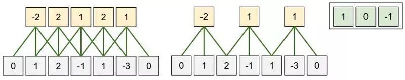
（关于 CNN 的说明 (摘自：http://cs231n.github.io/convolutional-networks/)

import pandas as pd
import numpy as numpy
from keras.models import Sequential
from keras.layers import Dense, Dropout, Activation, Flatten
from keras.layers import Conv1D, MaxPooling1D, LeakyReLU, PReLU
from keras.utils import np_utils
from keras.callbacks import CSVLogger, ModelCheckpoint
import h5py
import os
import tensorflow as tf
from keras.backend.tensorflow_backend import set_session
# Make the program use only one GPU
os.environ['CUDA_DEVICE_ORDER'] = 'PCI_BUS_ID'
os.environ['CUDA_VISIBLE_DEVICES'] = '1'
os.environ['TF_CPP_MIN_LOG_LEVEL']='2'
config = tf.ConfigProto()
config.gpu_options.allow_growth = True
set_session(tf.Session(config=config))
with h5py.File(''.join(['bitcoin2015to2017_close.h5']), 'r') as hf:
    datas = hf['inputs'].value
    labels = hf['outputs'].value
output_file_name='bitcoin2015to2017_close_CNN_2_relu'
step_size = datas.shape[1]
batch_size= 8
nb_features = datas.shape[2]
epochs = 100
#split training validation
training_size = int(0.8* datas.shape[0])
training_datas = datas[:training_size,:]
training_labels = labels[:training_size,:]
validation_datas = datas[training_size:,:]
validation_labels = labels[training_size:,:]
#build model
# 2 layers
model = Sequential()
model.add(Conv1D(activation='relu', input_shape=(step_size, nb_features), strides=3, filters=8, kernel_size=20))
model.add(Dropout(0.5))
model.add(Conv1D( strides=4, filters=nb_features, kernel_size=16))
'''
# 3 Layers
model.add(Conv1D(activation='relu', input_shape=(step_size, nb_features), strides=3, filters=8, kernel_size=8))
#model.add(LeakyReLU())
model.add(Dropout(0.5))
model.add(Conv1D(activation='relu', strides=2, filters=8, kernel_size=8))
#model.add(LeakyReLU())
model.add(Dropout(0.5))
model.add(Conv1D( strides=2, filters=nb_features, kernel_size=8))
# 4 layers
model.add(Conv1D(activation='relu', input_shape=(step_size, nb_features), strides=2, filters=8, kernel_size=2))
#model.add(LeakyReLU())
model.add(Dropout(0.5))
model.add(Conv1D(activation='relu', strides=2, filters=8, kernel_size=2))
#model.add(LeakyReLU())
model.add(Dropout(0.5))
model.add(Conv1D(activation='relu', strides=2, filters=8, kernel_size=2))
#model.add(LeakyReLU())
model.add(Dropout(0.5))
model.add(Conv1D( strides=2, filters=nb_features, kernel_size=2))
'''
model.compile(loss='mse', optimizer='adam')
model.fit(training_datas, training_labels,verbose=1, batch_size=batch_size,validation_data=(validation_datas,validation_labels), epochs = epochs, callbacks=[CSVLogger(output_file_name+'.csv', append=True),ModelCheckpoint('weights/'+output_file_name+'-{epoch:02d}-{val_loss:.5f}.hdf5', monitor='val_loss', verbose=1,mode='min')])

(原代码见 GitHub)

我建的第一个模型是 CNN。以下代码将 GPU 编号设置为“1”（因为我有 4 个，你可以将其设置为任何你喜欢的 GPU）。 由于 Tensorflow 在多 GPU 上运行情况似乎不太好，因此限制它只能在一个 GPU 上运行是明智的。如果你没有 GPU，请不要担心，直接忽略这段话就好了。

os.environ['CUDA_DEVICE_ORDER'] = 'PCI_BUS_ID' 
os.environ['CUDA_VISIBLE_DEVICES'] ='1' 
os.environ['TF_CPP_MIN_LOG_LEVEL']='2'

用于构建 CNN 模型的代码很简单。用 Dropout layer 来防止过度拟合的问题。定义损失函数为均方误差（Mean Squared Error，缩写为 MSE），优化器则选用目前最先进的 Adam。

model = Sequential() 
model.add(Conv1D(activation='relu', input_shape=(step_size, nb_features), strides=3, filters=8, kernel_size=20)) 
model.add(Dropout(0.5)) 
model.add(Conv1D( strides=4, filters=nb_features, kernel_size=16)) 
model.compile(loss='mse', optimizer='adam')

唯一一个你需要担心的是层与层间输入输出的维度问题。用于计算某个卷积层的公式是：

Output time step = (Input time step — Kernel size) / Strides + 1




在文件末尾，我添加了两个回调函数 CSVLogger 和 ModelCheckpoint。前者帮助我跟踪所有的训练和验证过程，而后者则允许我存储每个 epoch 的模型权重。

model.fit(training_datas, training_labels,verbose=1, batch_size=batch_size,validation_data=(validation_datas,validation_labels), epochs = epochs, callbacks=[CSVLogger(output_file_name+'.csv', append=True),ModelCheckpoint('weights/'+output_file_name+'-{epoch:02d}-{val_loss:.5f}.hdf5', monitor='val_loss', verbose=1,mode='min')]

 LSTM

长短期记忆（Long Short Term Memory，简写为 LSTM）网络是时间递归神经网络（Recurrent Neural Network，简写为 RNN）的一种变体（variation）。它被创造用来解决由 vanilla RNN 导致的梯度消失问题。据称，LSTM 能够用更长的时间步长（time step）来记住输入。

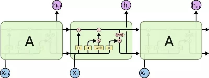
（LSTM 的说明，摘自：http://colah.github.io/posts/2015-08-Understanding-LSTMs/)

import pandas as pd
import numpy as numpy
from keras.models import Sequential
from keras.layers import Dense, Dropout, Activation, Flatten,Reshape
from keras.layers import Conv1D, MaxPooling1D
from keras.utils import np_utils
from keras.layers import LSTM, LeakyReLU
from keras.callbacks import CSVLogger, ModelCheckpoint
import h5py
import os
import tensorflow as tf
from keras.backend.tensorflow_backend import set_session
os.environ['CUDA_DEVICE_ORDER'] = 'PCI_BUS_ID'
os.environ['CUDA_VISIBLE_DEVICES'] = '1'
os.environ['TF_CPP_MIN_LOG_LEVEL']='2'
config = tf.ConfigProto()
config.gpu_options.allow_growth = True
set_session(tf.Session(config=config))
with h5py.File(''.join(['bitcoin2015to2017_close.h5']), 'r') as hf:
    datas = hf['inputs'].value
    labels = hf['outputs'].value
step_size = datas.shape[1]
units= 50
second_units = 30
batch_size = 8
nb_features = datas.shape[2]
epochs = 100
output_size=16
output_file_name='bitcoin2015to2017_close_LSTM_1_tanh_leaky_'
#split training validation
training_size = int(0.8* datas.shape[0])
training_datas = datas[:training_size,:]
training_labels = labels[:training_size,:,0]
validation_datas = datas[training_size:,:]
validation_labels = labels[training_size:,:,0]
#build model
model = Sequential()
model.add(LSTM(units=units,activation='tanh', input_shape=(step_size,nb_features),return_sequences=False))
model.add(Dropout(0.8))
model.add(Dense(output_size))
model.add(LeakyReLU())
model.compile(loss='mse', optimizer='adam')
model.fit(training_datas, training_labels, batch_size=batch_size,validation_data=(validation_datas,validation_labels), epochs = epochs, callbacks=[CSVLogger(output_file_name+'.csv', append=True),ModelCheckpoint('weights/'+output_file_name+'-{epoch:02d}-{val_loss:.5f}.hdf5', monitor='val_loss', verbose=1,mode='min')])

(原代码见 GitHub)

LSTM 比 CNN 更容易实现，因为你甚至不需要关心内核的大小、跨度、输入大小和输出大小之间的关系。只要确保输入和输出的维度在网络中定义是正确的。

model = Sequential() 
model.add(LSTM(units=units,activation='tanh', input_shape=(step_size,nb_features),return_sequences=False)) 
model.add(Dropout(0.8)) 
model.add(Dense(output_size)) 
model.add(LeakyReLU()) 
model.compile(loss='mse', optimizer='adam')

 GRU

GRU（Gated Recurrent Units）是 RNN 的另一种变体。它的网络结构不如 LSTM 那么复杂，只有一个 reset 和 forget gate，但是省略了内存单元。 据称，GRU 的性能与 LSTM 相当，但效率更高。（在这个博客中也是如此，因为 LSTM 大约需要 45 秒 /epoch，而 GRU 则不到 40 秒 /epoch）。

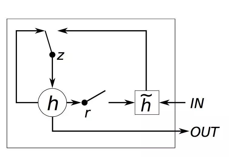
（关于 GRU 的说明，摘自：http://www.jackdermody.net/brightwire/article/GRU_Recurrent_Neural_Networks）

import pandas as pd
import numpy as numpy
from keras.models import Sequential
from keras.layers import Dense, Dropout, Activation, Flatten,Reshape
from keras.layers import Conv1D, MaxPooling1D, LeakyReLU
from keras.utils import np_utils
from keras.layers import GRU,CuDNNGRU
from keras.callbacks import CSVLogger, ModelCheckpoint
import h5py
import os
import tensorflow as tf
from keras.backend.tensorflow_backend import set_session
os.environ['CUDA_DEVICE_ORDER'] = 'PCI_BUS_ID'
os.environ['CUDA_VISIBLE_DEVICES'] = '1'
os.environ['TF_CPP_MIN_LOG_LEVEL']='2'
config = tf.ConfigProto()
config.gpu_options.allow_growth = True
set_session(tf.Session(config=config))
with h5py.File(''.join(['bitcoin2015to2017_close.h5']), 'r') as hf:
    datas = hf['inputs'].value
    labels = hf['outputs'].value
output_file_name='bitcoin2015to2017_close_GRU_1_tanh_relu_'
step_size = datas.shape[1]
units= 50
batch_size = 8
nb_features = datas.shape[2]
epochs = 100
output_size=16
#split training validation
training_size = int(0.8* datas.shape[0])
training_datas = datas[:training_size,:]
training_labels = labels[:training_size,:,0]
validation_datas = datas[training_size:,:]
validation_labels = labels[training_size:,:,0]
#build model
model = Sequential()
model.add(GRU(units=units, input_shape=(step_size,nb_features),return_sequences=False))
model.add(Activation('tanh'))
model.add(Dropout(0.2))
model.add(Dense(output_size))
model.add(Activation('relu'))
model.compile(loss='mse', optimizer='adam')
model.fit(training_datas, training_labels, batch_size=batch_size,validation_data=(validation_datas,validation_labels), epochs = epochs, callbacks=[CSVLogger(output_file_name+'.csv', append=True),ModelCheckpoint('weights/'+output_file_name+'-{epoch:02d}-{val_loss:.5f}.hdf5', monitor='val_loss', verbose=1,mode='min')])

(原代码见 GitHub)

仅需将正在建的 LSTM 模型代码中的第二行，

model.add(LSTM(units=units,activation='tanh', input_shape=(step_size,nb_features),return_sequences=False))




替换为：

model.add(GRU(units=units,activation='tanh', input_shape=(step_size,nb_features),return_sequences=False))




绘制结果图（result plotting）

由于三个模型的结果 de 绘图相似，所以这里我只放了 CNN 版本的图。首先，我们需要重新构建模型并将训练权重加载到模型中。

from keras import applications
from keras.models import Sequential
from keras.models import Model
from keras.layers import Dropout, Flatten, Dense, Activation
from keras.callbacks import CSVLogger
import tensorflow as tf
from scipy.ndimage import imread
import numpy as np
import random
from keras.layers import LSTM
from keras.layers import Conv1D, MaxPooling1D, LeakyReLU
from keras import backend as K
import keras
from keras.callbacks import CSVLogger, ModelCheckpoint
from keras.backend.tensorflow_backend import set_session
from keras import optimizers
import h5py
from sklearn.preprocessing import MinMaxScaler
import os
import pandas as pd
# import matplotlib
import matplotlib.pyplot as plt
os.environ['CUDA_DEVICE_ORDER'] = 'PCI_BUS_ID'
os.environ['CUDA_VISIBLE_DEVICES'] = '0'
os.environ['TF_CPP_MIN_LOG_LEVEL']='2'
with h5py.File(''.join(['bitcoin2015to2017_close.h5']), 'r') as hf:
    datas = hf['inputs'].value
    labels = hf['outputs'].value
    input_times = hf['input_times'].value
    output_times = hf['output_times'].value
    original_inputs = hf['original_inputs'].value
    original_outputs = hf['original_outputs'].value
    original_datas = hf['original_datas'].value
scaler=MinMaxScaler()
#split training validation
training_size = int(0.8* datas.shape[0])
training_datas = datas[:training_size,:,:]
training_labels = labels[:training_size,:,:]
validation_datas = datas[training_size:,:,:]
validation_labels = labels[training_size:,:,:]
validation_original_outputs = original_outputs[training_size:,:,:]
validation_original_inputs = original_inputs[training_size:,:,:]
validation_input_times = input_times[training_size:,:,:]
validation_output_times = output_times[training_size:,:,:]
ground_true = np.append(validation_original_inputs,validation_original_outputs, axis=1)
ground_true_times = np.append(validation_input_times,validation_output_times, axis=1)
step_size = datas.shape[1]
batch_size= 8
nb_features = datas.shape[2]
model = Sequential()
# 2 layers
model.add(Conv1D(activation='relu', input_shape=(step_size, nb_features), strides=3, filters=8, kernel_size=20))
# model.add(LeakyReLU())
model.add(Dropout(0.25))
model.add(Conv1D( strides=4, filters=nb_features, kernel_size=16))
model.load_weights('weights/bitcoin2015to2017_close_CNN_2_relu-44-0.00030.hdf5')
model.compile(loss='mse', optimizer='adam')

(原代码见 GitHub）

其次，我们需要对预测数据进行反向缩放，因为之前使用了 MinMaxScaler，所以预测的数据范围为 [0,1]。

predicted = model.predict(validation_datas)
predicted_inverted = []
for i in range(original_datas.shape[1]):
    scaler.fit(original_datas[:,i].reshape(-1,1))
    predicted_inverted.append(scaler.inverse_transform(predicted[:,:,i]))
print np.array(predicted_inverted).shape
#get only the close data
ground_true = ground_true[:,:,0].reshape(-1)
ground_true_times = ground_true_times.reshape(-1)
ground_true_times = pd.to_datetime(ground_true_times, unit='s')
# since we are appending in the first dimension
predicted_inverted = np.array(predicted_inverted)[0,:,:].reshape(-1)
print np.array(predicted_inverted).shape
validation_output_times = pd.to_datetime(validation_output_times.reshape(-1), unit='s')

(原代码见 GitHub）

建立两个 Dataframe 用于比特币的市场实际价格和预测价格。出于可视化的目的，绘制的数字仅显示了 2017 年 8 月之后的数据。

ground_true_df = pd.DataFrame()
ground_true_df['times'] = ground_true_times
ground_true_df['value'] = ground_true
prediction_df = pd.DataFrame()
prediction_df['times'] = validation_output_times
prediction_df['value'] = predicted_inverted
prediction_df = prediction_df.loc[(prediction_df["times"].dt.year == 2017 )&(prediction_df["times"].dt.month > 7 ),: ]
ground_true_df = ground_true_df.loc[(ground_true_df["times"].dt.year == 2017 )&(ground_true_df["times"].dt.month > 7 ),:]

(原代码见 GitHub）

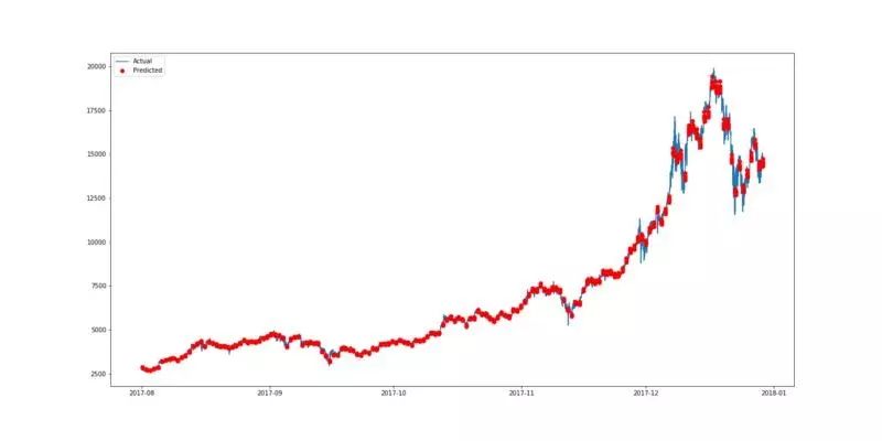
用 pyplot 来绘制图形。由于预测价格是基于每 16 分钟的基础上，所以将这些点分散会使我们更容易查看结果。因此，这里预测的数据被绘制为红点，如第三行中的“ro”所示。下图中的蓝线表示市场的真实情况（实际数据），而红点表示预测的比特币价格。

plt.figure(figsize=(20,10))
plt.plot(ground_true_df.times,ground_true_df.value, label = 'Actual')
plt.plot(prediction_df.times,prediction_df.value,'ro', label='Predicted')
plt.legend(loc='upper left')
plt.show()

（原代码见 GitHub）

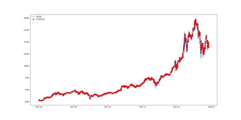
（用双层 CNN 预测比特币价格的最佳结果绘制）

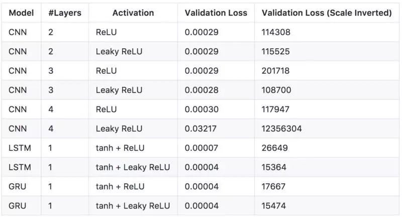
从上图可以看出，预测出的价格与比特币的实际价格非常相似。为了选择最佳模型，我决定测试几种不同的网络配置，也就有了下表。

（不同模型的预测结果）

上表中的每一行都是从总共 100 个训练 epoch 中导出的最佳验证损失（validation loss）的模型。从以上结果可以看出，LeakyReLU 似乎总是比正规的 ReLU 产生更好的损失（loss）。但是，使用 Leaky ReLU 作为激活函数的 4 层 CNN 会造成较大的验证损失。这可能是由于模型的错误部署造成的，对此可能需要进行重新的验证（re-validation）。CNN 模型可以训练得非常快（用 GPU，2 秒 /epoch），性能比 LSTM 和 GRU 稍差。 最好的模式似乎是 LSTM tanh 和 Leaky ReLU 作为激活函数，虽然 3 层 CNN 似乎能更好地捕捉局部临时的数据依赖性。

（有 tanh 函数和将 Leaky ReLu 作为激活函数的 LSTM）

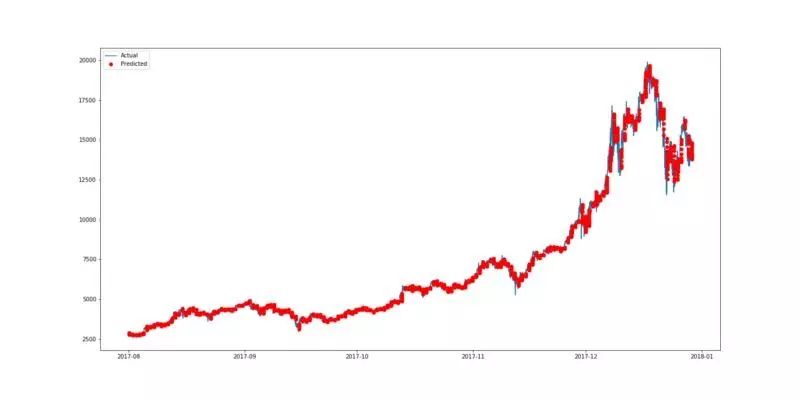
（以 Leaky ReLu 作为激活函数的 3 层 CNN）

虽然目前预测看起来相当不错，但是还是需要注意过度拟合的问题。训练和验证损失之间是有差距的（5.97E-06 vs 3.92E-05），在使用 LeakyReLU 进行 LSTM 训练时，应使用正则化（ regularization）来最小化差异。

正则化

为了找出最佳的正则化策略，我用几个不同的 L1 和 L2 值做了些试验。首先，需要定义一个新的函数来帮助我们将数据拟合成 LSTM。 在这里，我将以用偏差正则化器（bias regularizer）来正则化偏差向量为例。

def fit_lstm(reg):
    global training_datas, training_labels, batch_size, epochs,step_size,nb_features, units
    model = Sequential()
    model.add(CuDNNLSTM(units=units, bias_regularizer=reg, input_shape=(step_size,nb_features),return_sequences=False))
    model.add(Activation('tanh'))
    model.add(Dropout(0.2))
    model.add(Dense(output_size))
    model.add(LeakyReLU())
    model.compile(loss='mse', optimizer='adam')
    model.fit(training_datas, training_labels, batch_size=batch_size, epochs = epochs, verbose=0)
    return model

（原代码见 GitHub）

通过重复训练模型 30 次，每次用 30 个 epochs 进行试验。

def experiment(validation_datas,validation_labels,original_datas,ground_true,ground_true_times,validation_original_outputs, validation_output_times, nb_repeat, reg):
    error_scores = list()
    #get only the close data
    ground_true = ground_true[:,:,0].reshape(-1)
    ground_true_times = ground_true_times.reshape(-1)
    ground_true_times = pd.to_datetime(ground_true_times, unit='s')
    validation_output_times = pd.to_datetime(validation_output_times.reshape(-1), unit='s')
    for i in range(nb_repeat):
        model = fit_lstm(reg)
        predicted = model.predict(validation_datas)
        predicted_inverted = []
        scaler.fit(original_datas[:,0].reshape(-1,1))
        predicted_inverted.append(scaler.inverse_transform(predicted))
        # since we are appending in the first dimension
        predicted_inverted = np.array(predicted_inverted)[0,:,:].reshape(-1)
        error_scores.append(mean_squared_error(validation_original_outputs[:,:,0].reshape(-1),predicted_inverted))
    return error_scores
regs = [regularizers.l1(0),regularizers.l1(0.1), regularizers.l1(0.01), regularizers.l1(0.001), regularizers.l1(0.0001),regularizers.l2(0.1), regularizers.l2(0.01), regularizers.l2(0.001), regularizers.l2(0.0001)]
nb_repeat = 30
results = pd.DataFrame()
for reg in regs:
    name = ('l1 %.4f,l2 %.4f' % (reg.l1, reg.l2))
    print "Training "+ str(name)
    results[name] = experiment(validation_datas,validation_labels,original_datas,ground_true,ground_true_times,validation_original_outputs, validation_output_times, nb_repeat,reg)
results.describe().to_csv('result/lstm_bias_reg.csv')
results.describe()

（原代码见 GitHub）

如果你使用的是 Jupyter 笔记本，则可以直接从输出中查看下表。

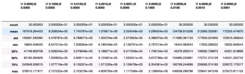
（偏差正则化器的运行结果）

为了可视化比较的结果，我们可以使用 boxplot：

results.describe().boxplot()
plt.show()

（原代码见 GitHub）

根据比较，偏差向量的系数为 0.01 的 L2 正则项（regularizers）似乎得到的结果最好。

为了找出所有正则项之间的最佳组合，包括激活、偏差、内核、循环矩阵，就必须要逐一地去测试这些正则项，就我目前使用的硬件配置而言还做不到。因此，我将把这个留待将来解决。

结论

通过这篇文章，你已经了解了：

• 如何收集实时比特币数据。

• 如何准备训练和测试用的数据。

• 如何使用深度学习预测比特币的价格。

• 如何可视化预测结果。

• 如何在模型上应用正则化。

今后这个博客的任务是找出最佳模型的最佳超参数（hyper-parameter），并可能会使用社交媒体来使预测的结果更为准确。这是我第一次在 Medium 中发布文章。如果有任何错误或问题，请不要犹豫，在下面留下你的评论。

更多有关信息，请参阅我的 github。

原文链接：

https://blog.goodaudience.com/predicting-cryptocurrency-price-with-tensorflow-and-keras-e1674b0dc58a