【复杂网络】经典网络建模

1. ER model

Generate two ER networks having 1000 and 10000 nodes with probability p = 3lnN/N, respectively.

def ER_Graph(N, p):
    graph = nx.Graph()

    for i in range(N):
        for j in range(i + 1, N):
            if random.random() < p:
                graph.add_edge(i, j)

    return graph

N1 = 1000
p1 = 3 * math.log(N1) / N1
G1 = ER_Graph(N1, p1)

N2 = 10000
p2 = 3 * math.log(N2) / N2
G2 = ER_Graph(N2, p2)

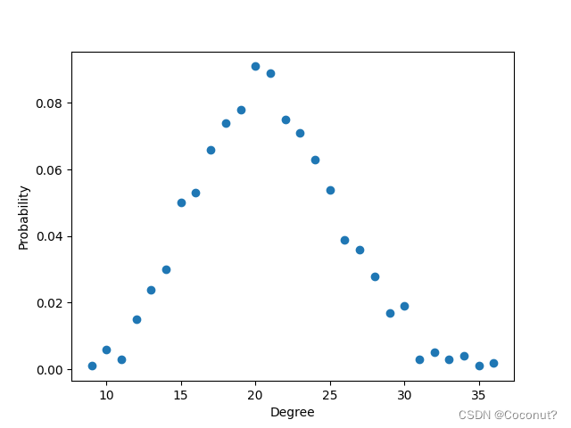
Properties for 1000 nodes:

• Average degree: 20.81
• Average shortest path: 2.614002002002002
• Average clustering: 0.02013893413807154
• Assortativity: -0.00151306936135126
• Degree distribution:
  

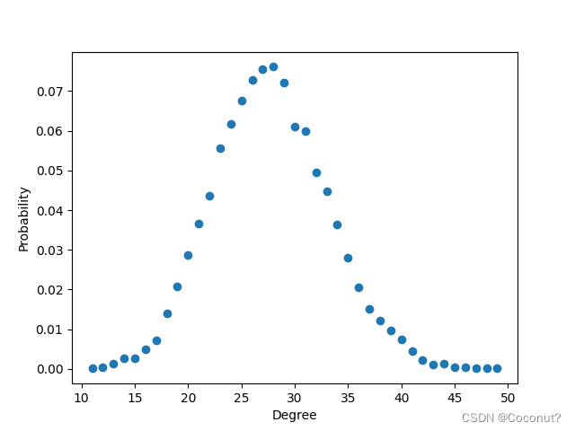
Properties for 10000 nodes:

• Average degree: 27.7232
• Average shortest path: 3.0491896989698968
• Average clustering: 0.0027163072614760373
• Assortativity: -0.0007480900331694497
• Degree distribution:

Theories:
$$<k>=p(N-1)$$$$P(k)=\left(\genfrac{}{}{0ex}{}{N-1}{k}\right)p^k(1-p{)}^{N-1-k}\approx \frac{<k{>}^k}{k!}{e}^{-<k>}$$$$<C>=p=\frac{<k>}{N-1}$$$$L\propto lnN/ln<k>$$$$Assortativity=r=\frac{cov(x_i,x_j)}{{\sigma }_x^2}$$

2. WS model

Generate a WS small-world network with N = 1000, p_{c} = 0.01.

def WS_Network(N, K, p_c):

    graph = nx.random_regular_graph(K, N)

    for u, v in graph.edges():
        if np.random.rand() < p_c:
            w = np.random.choice(N)
            while w == u or graph.has_edge(u, w):
                w = np.random.choice(N)
            graph.remove_edge(u, v)
            graph.add_edge(u, w)

    return graph

N = 1000
K = 10
p_c = 0.01
G = nx.watts_strogatz_graph(N, K, p_c)

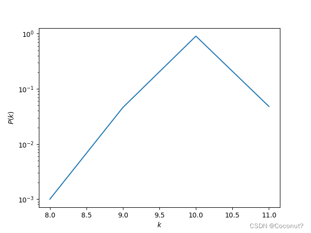
Properties:

• Average degree: 10.0
• Average shortest path: 8.869637637637638
• Average clustering: 0.6465472582972546
• Assortativity: 0.015456308253073254
• Degree distribution:
  

Theories:
$$<C>\approx \frac{3(K-2)}{4(K-1)}(1-p{)}^3$$$$L=\frac{N}{K}f(NKp)$$

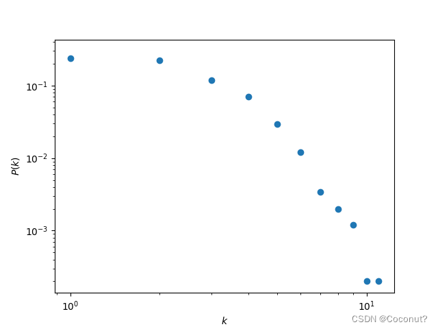
3. BA model

Generate a scale-free network with the BA model having 1000 nodes and m = 3.

def BA_Network(n, m):

    network = nx.Graph()
    network.add_nodes_from(range(m))
    target_list = list(range(m))
    source = m
    
    while source < n:
        targets = random.choices(target_list, k=m)
        network.add_node(source)
        network.add_edges_from([(source, target) for target in targets])
        target_list.extend([source] * m)
        target_list.extend(targets)
        source += 1
        
    return network

n = 1000
m = 3
G = BA_Network(n, m)

Properties:

• Average degree: 5.928
• Average shortest path: 3.4862522522522523
• Average clustering: 0.03115548822519195
• Assortativity: -0.08981049276336482
• Degree distribution:
  

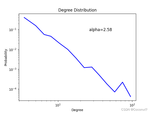
Theories:
$$k=2m$$$$P(k)=\frac{2m^2}{k^3}$$$$L\propto \frac{lnN}{lnlnN}$$$$<C>\propto \frac{(lnt{)}^2}{t}$$

4. Activity-driven model

Use activity-driven network to generated a temporal network with N = 5000, m = 2, g = 10, F(x) = x^(-c), c = 2.8.

def generate_activity_driven_network(N, m, g, c, lower_cut_off):
    network = nx.Graph()

    x = np.random.uniform(lower_cut_off, 1, N)
    F_x = x ** (-c)
    f_x = F_x / np.sum(F_x)
    
    for i in range(N):
        network.add_node(i)

    for step in range(t):
       
        temp_network = nx.Graph()
        
        for i in range(N):
            temp_network.add_node(i) 
       
        for i in range(N):

            selected_x = np.random.choice(x, size=1, p=f_x)
            a = g * selected_x

            if random.uniform(0, 1) < a:  
                for _ in range(m):
                    valid_nodes = list(set(range(N)) - set(temp_network.neighbors(i)))  
                    if len(valid_nodes) == 0:  
                        break
                    j = np.random.choice(valid_nodes)
                    temp_network.add_edge(i, j)

        network = nx.compose(network, temp_network)

    return network

N = 5000 
m = 2 
g = 10 
c = 2.8 
t = 20  
lower_cut_off = 0.001 
integrated_network = generate_activity_driven_network(N, m, g, c, lower_cut_off)

Properties of the integrated network:

• Average degree: 1.5568
• Largest giant component: 3202
• Degree distribution: