


目录
3.1均方误差:mse = mean_squared_error(y真实值,y预测值)
3.2均方根误差:rmse = (mean_squared_error(y真实值,y预测值))**0.5
3.3平均绝对值误差:mae = mean_absolute_error(y真实值,y预测值)
3.4r2打分:r2 = r2_score(y真实值,y预测值) 或者r2=lr.score(x真实值,y真实值)
1.什么是线性回归
两个变量之间存在一次方函数关系,就称它们之间存在线性关系。更通俗一点讲,如果把这两个变量分别作为点的横坐标与纵坐标,其图象是平面上的一条直线,则这两个变量之间的关系就是线性关系。
2.线性回归思路
"""
1.获取数据集
2.指定特征值x、目标值y(想获得什么数据,预测什么数据就设为y)
3.数据集划分:训练集(默认75%)和测试集(默认25%)
4.建立模型、拟合、预测
5.模型评估

预测结果:          出太阳     出太阳     下雨
测试集的真实结果:   阴天      出太阳     下雨
正确率为66.66%
"""
3.几种回归模型评估

3.1均方误差:mse = mean_squared_error(y真实值,y预测值)

误差越接近0,误差越小
3.2均方根误差:rmse = (mean_squared_error(y真实值,y预测值))**0.5

误差越接近0,误差越小
3.3平均绝对值误差:mae = mean_absolute_error(y真实值,y预测值)

误差越接近0,误差越小
3.4r2打分:r2 = r2_score(y真实值,y预测值) 或者r2=lr.score(x真实值,y真实值)


分数越高表示越好
4.单(一)元线性回归
# 安装pip install scikit-learn
#线性回归类
from sklearn.linear_model import LinearRegression
# 数据集划分
from sklearn.model_selection import train_test_split
#数据集
from sklearn.datasets import load_iris
# 单(一)元线性回归
# 获取数据集
iris = load_iris()
print('iris原始数据:',iris)
print('*'*100)
# 指定特征列x,y
x,y = iris.data[:,2].reshape(-1,1),iris.data[:,3].reshape(-1,1)
print('x数据:',x)
print('*'*60)
print('y数据:',y)
print('*'*40)
"""
# 随机种子
import random
# 5就是随机种子
random.seed(5)
num = [random.randint(1,100)for i in range(5)]
print(num)
# 划分训练集和测试集,把数据源给train_test_split,系统自行分割,
0.2是测试集的比例,random_state随机种子,数字是自定义,
数字不一样评估结果可能不一样,可以调
"""
x_train,x_test,y_train,y_test = train_test_split(x,y,test_size=0.2,random_state=2)
# 建立模型
lr = LinearRegression()
#拟合,计算方程参数w和b,y=w*x+b,系统自行计算
lr.fit(x_train,y_train)
print('权重w:',lr.coef_)
print('*'*30)
print('截距b:',lr.intercept_)
print('*'*30)
# 预测
y_hat = lr.predict(x_test) #模型训练出来然后用测试值去测试出来的结果
print('y_hat预测数据:',y_hat[:5])
print('*'*30)
print('y_text真实数据:',y_test[:5]) # 真实值
print('*'*40)
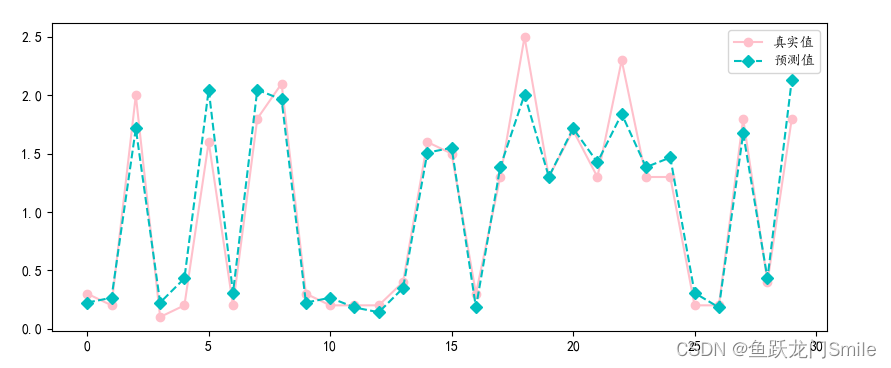
# 图形模型评估
import matplotlib.pyplot as plt
plt.rcParams['font.family']=['KaiTi']
plt.figure(figsize=(10,4))
plt.plot(y_test,label='真实值',color='pink',marker='o')
plt.plot(y_hat,label='预测值',color='c',marker='D',ls='--')
plt.legend()
plt.show()
# 导入回归模型评估
from sklearn.metrics import mean_squared_error,mean_absolute_error,r2_score
#越接近于0,误差越小
# 均方误差0.03810129178169931
mse = mean_squared_error(y_test,y_hat)
print('均方误差mse:',mse)
print('*'*40)
# 均方根误差0.19519552193044623
rmse = mse**0.5
print('均方根误差rmse:',rmse)
print('*'*40)
#平均绝对值误差0.1430440743648432
mae = mean_absolute_error(y_test,y_hat)
print('平均绝对值误差mae:',mae)
print('*'*40)
#r2分数,打分0.9368067916048772,93.68很好了
r2 = r2_score(y_test,y_hat)
print('r2打分:',r2)
# 另一种r2打分方法
print('另一种r2打分方法:',lr.score(x_test, y_test))运行结果:
iris原始数据:
{'data': array([[5.1, 3.5, 1.4, 0.2],
       [4.9, 3. , 1.4, 0.2],
       [4.7, 3.2, 1.3, 0.2],
       [4.6, 3.1, 1.5, 0.2],
       [5. , 3.6, 1.4, 0.2],
       [5.4, 3.9, 1.7, 0.4],
       [4.6, 3.4, 1.4, 0.3],
       [5. , 3.4, 1.5, 0.2],
       [4.4, 2.9, 1.4, 0.2],
       [4.9, 3.1, 1.5, 0.1],
       [5.4, 3.7, 1.5, 0.2],
       [4.8, 3.4, 1.6, 0.2],
       [4.8, 3. , 1.4, 0.1],
       [4.3, 3. , 1.1, 0.1],
       [5.8, 4. , 1.2, 0.2],
       [5.7, 4.4, 1.5, 0.4],
       [5.4, 3.9, 1.3, 0.4],
       [5.1, 3.5, 1.4, 0.3],
       [5.7, 3.8, 1.7, 0.3],
       [5.1, 3.8, 1.5, 0.3],
       [5.4, 3.4, 1.7, 0.2],
       [5.1, 3.7, 1.5, 0.4],
       [4.6, 3.6, 1. , 0.2],
       [5.1, 3.3, 1.7, 0.5],
       [4.8, 3.4, 1.9, 0.2],
       [5. , 3. , 1.6, 0.2],
       [5. , 3.4, 1.6, 0.4],
       [5.2, 3.5, 1.5, 0.2],
       [5.2, 3.4, 1.4, 0.2],
       [4.7, 3.2, 1.6, 0.2],
       [4.8, 3.1, 1.6, 0.2],
       [5.4, 3.4, 1.5, 0.4],
       [5.2, 4.1, 1.5, 0.1],
       [5.5, 4.2, 1.4, 0.2],
       [4.9, 3.1, 1.5, 0.2],
       [5. , 3.2, 1.2, 0.2],
       [5.5, 3.5, 1.3, 0.2],
       [4.9, 3.6, 1.4, 0.1],
       [4.4, 3. , 1.3, 0.2],
       [5.1, 3.4, 1.5, 0.2],
       [5. , 3.5, 1.3, 0.3],
       [4.5, 2.3, 1.3, 0.3],
       [4.4, 3.2, 1.3, 0.2],
       [5. , 3.5, 1.6, 0.6],
       [5.1, 3.8, 1.9, 0.4],
       [4.8, 3. , 1.4, 0.3],
       [5.1, 3.8, 1.6, 0.2],
       [4.6, 3.2, 1.4, 0.2],
       [5.3, 3.7, 1.5, 0.2],
       [5. , 3.3, 1.4, 0.2],
       [7. , 3.2, 4.7, 1.4],
       [6.4, 3.2, 4.5, 1.5],
       [6.9, 3.1, 4.9, 1.5],
       [5.5, 2.3, 4. , 1.3],
       [6.5, 2.8, 4.6, 1.5],
       [5.7, 2.8, 4.5, 1.3],
       [6.3, 3.3, 4.7, 1.6],
       [4.9, 2.4, 3.3, 1. ],
       [6.6, 2.9, 4.6, 1.3],
       [5.2, 2.7, 3.9, 1.4],
       [5. , 2. , 3.5, 1. ],
       [5.9, 3. , 4.2, 1.5],
       [6. , 2.2, 4. , 1. ],
       [6.1, 2.9, 4.7, 1.4],
       [5.6, 2.9, 3.6, 1.3],
       [6.7, 3.1, 4.4, 1.4],
       [5.6, 3. , 4.5, 1.5],
       [5.8, 2.7, 4.1, 1. ],
       [6.2, 2.2, 4.5, 1.5],
       [5.6, 2.5, 3.9, 1.1],
       [5.9, 3.2, 4.8, 1.8],
       [6.1, 2.8, 4. , 1.3],
       [6.3, 2.5, 4.9, 1.5],
       [6.1, 2.8, 4.7, 1.2],
       [6.4, 2.9, 4.3, 1.3],
       [6.6, 3. , 4.4, 1.4],
       [6.8, 2.8, 4.8, 1.4],
       [6.7, 3. , 5. , 1.7],
       [6. , 2.9, 4.5, 1.5],
       [5.7, 2.6, 3.5, 1. ],
       [5.5, 2.4, 3.8, 1.1],
       [5.5, 2.4, 3.7, 1. ],
       [5.8, 2.7, 3.9, 1.2],
       [6. , 2.7, 5.1, 1.6],
       [5.4, 3. , 4.5, 1.5],
       [6. , 3.4, 4.5, 1.6],
       [6.7, 3.1, 4.7, 1.5],
       [6.3, 2.3, 4.4, 1.3],
       [5.6, 3. , 4.1, 1.3],
       [5.5, 2.5, 4. , 1.3],
       [5.5, 2.6, 4.4, 1.2],
       [6.1, 3. , 4.6, 1.4],
       [5.8, 2.6, 4. , 1.2],
       [5. , 2.3, 3.3, 1. ],
       [5.6, 2.7, 4.2, 1.3],
       [5.7, 3. , 4.2, 1.2],
       [5.7, 2.9, 4.2, 1.3],
       [6.2, 2.9, 4.3, 1.3],
       [5.1, 2.5, 3. , 1.1],
       [5.7, 2.8, 4.1, 1.3],
       [6.3, 3.3, 6. , 2.5],
       [5.8, 2.7, 5.1, 1.9],
       [7.1, 3. , 5.9, 2.1],
       [6.3, 2.9, 5.6, 1.8],
       [6.5, 3. , 5.8, 2.2],
       [7.6, 3. , 6.6, 2.1],
       [4.9, 2.5, 4.5, 1.7],
       [7.3, 2.9, 6.3, 1.8],
       [6.7, 2.5, 5.8, 1.8],
       [7.2, 3.6, 6.1, 2.5],
       [6.5, 3.2, 5.1, 2. ],
       [6.4, 2.7, 5.3, 1.9],
       [6.8, 3. , 5.5, 2.1],
       [5.7, 2.5, 5. , 2. ],
       [5.8, 2.8, 5.1, 2.4],
       [6.4, 3.2, 5.3, 2.3],
       [6.5, 3. , 5.5, 1.8],
       [7.7, 3.8, 6.7, 2.2],
       [7.7, 2.6, 6.9, 2.3],
       [6. , 2.2, 5. , 1.5],
       [6.9, 3.2, 5.7, 2.3],
       [5.6, 2.8, 4.9, 2. ],
       [7.7, 2.8, 6.7, 2. ],
       [6.3, 2.7, 4.9, 1.8],
       [6.7, 3.3, 5.7, 2.1],
       [7.2, 3.2, 6. , 1.8],
       [6.2, 2.8, 4.8, 1.8],
       [6.1, 3. , 4.9, 1.8],
       [6.4, 2.8, 5.6, 2.1],
       [7.2, 3. , 5.8, 1.6],
       [7.4, 2.8, 6.1, 1.9],
       [7.9, 3.8, 6.4, 2. ],
       [6.4, 2.8, 5.6, 2.2],
       [6.3, 2.8, 5.1, 1.5],
       [6.1, 2.6, 5.6, 1.4],
       [7.7, 3. , 6.1, 2.3],
       [6.3, 3.4, 5.6, 2.4],
       [6.4, 3.1, 5.5, 1.8],
       [6. , 3. , 4.8, 1.8],
       [6.9, 3.1, 5.4, 2.1],
       [6.7, 3.1, 5.6, 2.4],
       [6.9, 3.1, 5.1, 2.3],
       [5.8, 2.7, 5.1, 1.9],
       [6.8, 3.2, 5.9, 2.3],
       [6.7, 3.3, 5.7, 2.5],
       [6.7, 3. , 5.2, 2.3],
       [6.3, 2.5, 5. , 1.9],
       [6.5, 3. , 5.2, 2. ],
       [6.2, 3.4, 5.4, 2.3],
       [5.9, 3. , 5.1, 1.8]]),
'target': array([0, 0, 0, 0, 0, 0, 0, 0, 0, 0, 0, 0, 0, 0, 0, 0, 0, 0, 0, 0, 0, 0,
       0, 0, 0, 0, 0, 0, 0, 0, 0, 0, 0, 0, 0, 0, 0, 0, 0, 0, 0, 0, 0, 0,
       0, 0, 0, 0, 0, 0, 1, 1, 1, 1, 1, 1, 1, 1, 1, 1, 1, 1, 1, 1, 1, 1,
       1, 1, 1, 1, 1, 1, 1, 1, 1, 1, 1, 1, 1, 1, 1, 1, 1, 1, 1, 1, 1, 1,
       1, 1, 1, 1, 1, 1, 1, 1, 1, 1, 1, 1, 2, 2, 2, 2, 2, 2, 2, 2, 2, 2,
       2, 2, 2, 2, 2, 2, 2, 2, 2, 2, 2, 2, 2, 2, 2, 2, 2, 2, 2, 2, 2, 2,
       2, 2, 2, 2, 2, 2, 2, 2, 2, 2, 2, 2, 2, 2, 2, 2, 2, 2]), 'frame': None, 'target_names': array(['setosa', 'versicolor', 'virginica'], dtype='<U10'), 'DESCR': '.. _iris_dataset:\n\nIris plants dataset\n--------------------\n\n**Data Set Characteristics:**\n\n:Number of Instances: 150 (50 in each of three classes)\n:Number of Attributes: 4 numeric, predictive attributes and the class\n:Attribute Information:\n    - sepal length in cm\n    - sepal width in cm\n    - petal length in cm\n    - petal width in cm\n    - class:\n            - Iris-Setosa\n            - Iris-Versicolour\n            - Iris-Virginica\n\n:Summary Statistics:\n\n============== ==== ==== ======= ===== ====================\n                Min  Max   Mean    SD   Class Correlation\n============== ==== ==== ======= ===== ====================\nsepal length:   4.3  7.9   5.84   0.83    0.7826\nsepal width:    2.0  4.4   3.05   0.43   -0.4194\npetal length:   1.0  6.9   3.76   1.76    0.9490  (high!)\npetal width:    0.1  2.5   1.20   0.76    0.9565  (high!)\n============== ==== ==== ======= ===== ====================\n\n:Missing Attribute Values: None\n:Class Distribution: 33.3% for each of 3 classes.\n:Creator: R.A. Fisher\n:Donor: Michael Marshall (MARSHALL%PLU@io.arc.nasa.gov)\n:Date: July, 1988\n\nThe famous Iris database, first used by Sir R.A. Fisher. The dataset is taken\nfrom Fisher\'s paper. Note that it\'s the same as in R, but not as in the UCI\nMachine Learning Repository, which has two wrong data points.\n\nThis is perhaps the best known database to be found in the\npattern recognition literature.  Fisher\'s paper is a classic in the field and\nis referenced frequently to this day.  (See Duda & Hart, for example.)  The\ndata set contains 3 classes of 50 instances each, where each class refers to a\ntype of iris plant.  One class is linearly separable from the other 2; the\nlatter are NOT linearly separable from each other.\n\n|details-start|\n**References**\n|details-split|\n\n- Fisher, R.A. "The use of multiple measurements in taxonomic problems"\n  Annual Eugenics, 7, Part II, 179-188 (1936); also in "Contributions to\n  Mathematical Statistics" (John Wiley, NY, 1950).\n- Duda, R.O., & Hart, P.E. (1973) Pattern Classification and Scene Analysis.\n  (Q327.D83) John Wiley & Sons.  ISBN 0-471-22361-1.  See page 218.\n- Dasarathy, B.V. (1980) "Nosing Around the Neighborhood: A New System\n  Structure and Classification Rule for Recognition in Partially Exposed\n  Environments".  IEEE Transactions on Pattern Analysis and Machine\n  Intelligence, Vol. PAMI-2, No. 1, 67-71.\n- Gates, G.W. (1972) "The Reduced Nearest Neighbor Rule".  IEEE Transactions\n  on Information Theory, May 1972, 431-433.\n- See also: 1988 MLC Proceedings, 54-64.  Cheeseman et al"s AUTOCLASS II\n  conceptual clustering system finds 3 classes in the data.\n- Many, many more ...\n\n|details-end|\n', 'feature_names': ['sepal length (cm)', 'sepal width (cm)', 'petal length (cm)', 'petal width (cm)'], 'filename': 'iris.csv', 'data_module': 'sklearn.datasets.data'}
****************************************************************************************************
x数据:
[[1.4]
 [1.4]
 [1.3]
 [1.5]
 [1.4]
 [1.7]
 [1.4]
 [1.5]
 [1.4]
 [1.5]
 [1.5]
 [1.6]
 [1.4]
 [1.1]
 [1.2]
 [1.5]
 [1.3]
 [1.4]
 [1.7]
 [1.5]
 [1.7]
 [1.5]
 [1. ]
 [1.7]
 [1.9]
 [1.6]
 [1.6]
 [1.5]
 [1.4]
 [1.6]
 [1.6]
 [1.5]
 [1.5]
 [1.4]
 [1.5]
 [1.2]
 [1.3]
 [1.4]
 [1.3]
 [1.5]
 [1.3]
 [1.3]
 [1.3]
 [1.6]
 [1.9]
 [1.4]
 [1.6]
 [1.4]
 [1.5]
 [1.4]
 [4.7]
 [4.5]
 [4.9]
 [4. ]
 [4.6]
 [4.5]
 [4.7]
 [3.3]
 [4.6]
 [3.9]
 [3.5]
 [4.2]
 [4. ]
 [4.7]
 [3.6]
 [4.4]
 [4.5]
 [4.1]
 [4.5]
 [3.9]
 [4.8]
 [4. ]
 [4.9]
 [4.7]
 [4.3]
 [4.4]
 [4.8]
 [5. ]
 [4.5]
 [3.5]
 [3.8]
 [3.7]
 [3.9]
 [5.1]
 [4.5]
 [4.5]
 [4.7]
 [4.4]
 [4.1]
 [4. ]
 [4.4]
 [4.6]
 [4. ]
 [3.3]
 [4.2]
 [4.2]
 [4.2]
 [4.3]
 [3. ]
 [4.1]
 [6. ]
 [5.1]
 [5.9]
 [5.6]
 [5.8]
 [6.6]
 [4.5]
 [6.3]
 [5.8]
 [6.1]
 [5.1]
 [5.3]
 [5.5]
 [5. ]
 [5.1]
 [5.3]
 [5.5]
 [6.7]
 [6.9]
 [5. ]
 [5.7]
 [4.9]
 [6.7]
 [4.9]
 [5.7]
 [6. ]
 [4.8]
 [4.9]
 [5.6]
 [5.8]
 [6.1]
 [6.4]
 [5.6]
 [5.1]
 [5.6]
 [6.1]
 [5.6]
 [5.5]
 [4.8]
 [5.4]
 [5.6]
 [5.1]
 [5.1]
 [5.9]
 [5.7]
 [5.2]
 [5. ]
 [5.2]
 [5.4]
 [5.1]]
************************************************************
y数据:
[[0.2]
 [0.2]
 [0.2]
 [0.2]
 [0.2]
 [0.4]
 [0.3]
 [0.2]
 [0.2]
 [0.1]
 [0.2]
 [0.2]
 [0.1]
 [0.1]
 [0.2]
 [0.4]
 [0.4]
 [0.3]
 [0.3]
 [0.3]
 [0.2]
 [0.4]
 [0.2]
 [0.5]
 [0.2]
 [0.2]
 [0.4]
 [0.2]
 [0.2]
 [0.2]
 [0.2]
 [0.4]
 [0.1]
 [0.2]
 [0.2]
 [0.2]
 [0.2]
 [0.1]
 [0.2]
 [0.2]
 [0.3]
 [0.3]
 [0.2]
 [0.6]
 [0.4]
 [0.3]
 [0.2]
 [0.2]
 [0.2]
 [0.2]
 [1.4]
 [1.5]
 [1.5]
 [1.3]
 [1.5]
 [1.3]
 [1.6]
 [1. ]
 [1.3]
 [1.4]
 [1. ]
 [1.5]
 [1. ]
 [1.4]
 [1.3]
 [1.4]
 [1.5]
 [1. ]
 [1.5]
 [1.1]
 [1.8]
 [1.3]
 [1.5]
 [1.2]
 [1.3]
 [1.4]
 [1.4]
 [1.7]
 [1.5]
 [1. ]
 [1.1]
 [1. ]
 [1.2]
 [1.6]
 [1.5]
 [1.6]
 [1.5]
 [1.3]
 [1.3]
 [1.3]
 [1.2]
 [1.4]
 [1.2]
 [1. ]
 [1.3]
 [1.2]
 [1.3]
 [1.3]
 [1.1]
 [1.3]
 [2.5]
 [1.9]
 [2.1]
 [1.8]
 [2.2]
 [2.1]
 [1.7]
 [1.8]
 [1.8]
 [2.5]
 [2. ]
 [1.9]
 [2.1]
 [2. ]
 [2.4]
 [2.3]
 [1.8]
 [2.2]
 [2.3]
 [1.5]
 [2.3]
 [2. ]
 [2. ]
 [1.8]
 [2.1]
 [1.8]
 [1.8]
 [1.8]
 [2.1]
 [1.6]
 [1.9]
 [2. ]
 [2.2]
 [1.5]
 [1.4]
 [2.3]
 [2.4]
 [1.8]
 [1.8]
 [2.1]
 [2.4]
 [2.3]
 [1.9]
 [2.3]
 [2.5]
 [2.3]
 [1.9]
 [2. ]
 [2.3]
 [1.8]]
****************************************
权重w: [[0.4145955]]
******************************
截距b: [-0.35686296]
******************************
y_hat预测数据:
[[0.22357074]
 [0.26503029]
 [1.71611455]
 [0.22357074]
 [0.43086849]]
******************************
y_text真实数据:
[[0.3]
 [0.2]
 [2. ]
 [0.1]
 [0.2]]
****************************************
均方误差mse: 0.03810129178169931
****************************************
均方根误差rmse: 0.19519552193044623
****************************************
平均绝对值误差mae: 0.1430440743648432
****************************************
r2打分: 0.9368067916048772
另一种r2打分方法: 0.9368067916048772
5.多元线性回归
# 安装pip install scikit-learn
#线性回归类
from sklearn.linear_model import LinearRegression
# 数据集划分
from sklearn.model_selection import train_test_split
#数据集
from sklearn.datasets import load_iris

# 多元线性回归
#获取数据集
iris = load_iris()
print('iris原始数据:')
print(iris)
print('*'*100)
#设定特征值,xy
x,y = iris.data,iris.target.reshape(-1,1)
#x为多元
print('x数据为:',x)
print('x长度为:',len(x))
print('*'*50)
print('y数据为:',y)
print('y长度为:',len(y))
print('*'*50)

# 划分训练集和测试集
x_train,x_test,y_train,y_test = train_test_split(x,y,test_size=0.2,random_state=2)

# 建立模型
lr = LinearRegression()

#拟合,计算w和b
lr.fit(x_train,y_train)
w = lr.coef_
print('权重w的值:')
print(w)
b = lr.intercept_
print('截距b的值:')
print(b)
print('*'*50)

#预测
y_hat = lr.predict(x_test)
print('y_hat预测值:')
print(y_hat[:10])
print('y_test真实值:')
print(y_test[:10])
print('*'*40)

# 导入回归模型评估
from sklearn.metrics import mean_squared_error,mean_absolute_error,r2_score
mse = mean_squared_error(y_test,y_hat)
print('均方误差mse:')
print(mse)
print('*'*40)

rmse = mse**0.5
print('均方根误差rmse:')
print(rmse)
print('*'*40)


mae = mean_absolute_error(y_test,y_hat)
print('平绝对值误差:')
print(mae)
print('*'*40)
r2 = r2_score(y_test,y_hat)
print('r2打分:')
print(r2)
print('另一种r2打分:')
print(lr.score(x_test,y_test))
运行结果:
iris原始数据:
{'data': array([[5.1, 3.5, 1.4, 0.2],
       [4.9, 3. , 1.4, 0.2],
       [4.7, 3.2, 1.3, 0.2],
       [4.6, 3.1, 1.5, 0.2],
       [5. , 3.6, 1.4, 0.2],
       [5.4, 3.9, 1.7, 0.4],
       [4.6, 3.4, 1.4, 0.3],
       [5. , 3.4, 1.5, 0.2],
       [4.4, 2.9, 1.4, 0.2],
       [4.9, 3.1, 1.5, 0.1],
       [5.4, 3.7, 1.5, 0.2],
       [4.8, 3.4, 1.6, 0.2],
       [4.8, 3. , 1.4, 0.1],
       [4.3, 3. , 1.1, 0.1],
       [5.8, 4. , 1.2, 0.2],
       [5.7, 4.4, 1.5, 0.4],
       [5.4, 3.9, 1.3, 0.4],
       [5.1, 3.5, 1.4, 0.3],
       [5.7, 3.8, 1.7, 0.3],
       [5.1, 3.8, 1.5, 0.3],
       [5.4, 3.4, 1.7, 0.2],
       [5.1, 3.7, 1.5, 0.4],
       [4.6, 3.6, 1. , 0.2],
       [5.1, 3.3, 1.7, 0.5],
       [4.8, 3.4, 1.9, 0.2],
       [5. , 3. , 1.6, 0.2],
       [5. , 3.4, 1.6, 0.4],
       [5.2, 3.5, 1.5, 0.2],
       [5.2, 3.4, 1.4, 0.2],
       [4.7, 3.2, 1.6, 0.2],
       [4.8, 3.1, 1.6, 0.2],
       [5.4, 3.4, 1.5, 0.4],
       [5.2, 4.1, 1.5, 0.1],
       [5.5, 4.2, 1.4, 0.2],
       [4.9, 3.1, 1.5, 0.2],
       [5. , 3.2, 1.2, 0.2],
       [5.5, 3.5, 1.3, 0.2],
       [4.9, 3.6, 1.4, 0.1],
       [4.4, 3. , 1.3, 0.2],
       [5.1, 3.4, 1.5, 0.2],
       [5. , 3.5, 1.3, 0.3],
       [4.5, 2.3, 1.3, 0.3],
       [4.4, 3.2, 1.3, 0.2],
       [5. , 3.5, 1.6, 0.6],
       [5.1, 3.8, 1.9, 0.4],
       [4.8, 3. , 1.4, 0.3],
       [5.1, 3.8, 1.6, 0.2],
       [4.6, 3.2, 1.4, 0.2],
       [5.3, 3.7, 1.5, 0.2],
       [5. , 3.3, 1.4, 0.2],
       [7. , 3.2, 4.7, 1.4],
       [6.4, 3.2, 4.5, 1.5],
       [6.9, 3.1, 4.9, 1.5],
       [5.5, 2.3, 4. , 1.3],
       [6.5, 2.8, 4.6, 1.5],
       [5.7, 2.8, 4.5, 1.3],
       [6.3, 3.3, 4.7, 1.6],
       [4.9, 2.4, 3.3, 1. ],
       [6.6, 2.9, 4.6, 1.3],
       [5.2, 2.7, 3.9, 1.4],
       [5. , 2. , 3.5, 1. ],
       [5.9, 3. , 4.2, 1.5],
       [6. , 2.2, 4. , 1. ],
       [6.1, 2.9, 4.7, 1.4],
       [5.6, 2.9, 3.6, 1.3],
       [6.7, 3.1, 4.4, 1.4],
       [5.6, 3. , 4.5, 1.5],
       [5.8, 2.7, 4.1, 1. ],
       [6.2, 2.2, 4.5, 1.5],
       [5.6, 2.5, 3.9, 1.1],
       [5.9, 3.2, 4.8, 1.8],
       [6.1, 2.8, 4. , 1.3],
       [6.3, 2.5, 4.9, 1.5],
       [6.1, 2.8, 4.7, 1.2],
       [6.4, 2.9, 4.3, 1.3],
       [6.6, 3. , 4.4, 1.4],
       [6.8, 2.8, 4.8, 1.4],
       [6.7, 3. , 5. , 1.7],
       [6. , 2.9, 4.5, 1.5],
       [5.7, 2.6, 3.5, 1. ],
       [5.5, 2.4, 3.8, 1.1],
       [5.5, 2.4, 3.7, 1. ],
       [5.8, 2.7, 3.9, 1.2],
       [6. , 2.7, 5.1, 1.6],
       [5.4, 3. , 4.5, 1.5],
       [6. , 3.4, 4.5, 1.6],
       [6.7, 3.1, 4.7, 1.5],
       [6.3, 2.3, 4.4, 1.3],
       [5.6, 3. , 4.1, 1.3],
       [5.5, 2.5, 4. , 1.3],
       [5.5, 2.6, 4.4, 1.2],
       [6.1, 3. , 4.6, 1.4],
       [5.8, 2.6, 4. , 1.2],
       [5. , 2.3, 3.3, 1. ],
       [5.6, 2.7, 4.2, 1.3],
       [5.7, 3. , 4.2, 1.2],
       [5.7, 2.9, 4.2, 1.3],
       [6.2, 2.9, 4.3, 1.3],
       [5.1, 2.5, 3. , 1.1],
       [5.7, 2.8, 4.1, 1.3],
       [6.3, 3.3, 6. , 2.5],
       [5.8, 2.7, 5.1, 1.9],
       [7.1, 3. , 5.9, 2.1],
       [6.3, 2.9, 5.6, 1.8],
       [6.5, 3. , 5.8, 2.2],
       [7.6, 3. , 6.6, 2.1],
       [4.9, 2.5, 4.5, 1.7],
       [7.3, 2.9, 6.3, 1.8],
       [6.7, 2.5, 5.8, 1.8],
       [7.2, 3.6, 6.1, 2.5],
       [6.5, 3.2, 5.1, 2. ],
       [6.4, 2.7, 5.3, 1.9],
       [6.8, 3. , 5.5, 2.1],
       [5.7, 2.5, 5. , 2. ],
       [5.8, 2.8, 5.1, 2.4],
       [6.4, 3.2, 5.3, 2.3],
       [6.5, 3. , 5.5, 1.8],
       [7.7, 3.8, 6.7, 2.2],
       [7.7, 2.6, 6.9, 2.3],
       [6. , 2.2, 5. , 1.5],
       [6.9, 3.2, 5.7, 2.3],
       [5.6, 2.8, 4.9, 2. ],
       [7.7, 2.8, 6.7, 2. ],
       [6.3, 2.7, 4.9, 1.8],
       [6.7, 3.3, 5.7, 2.1],
       [7.2, 3.2, 6. , 1.8],
       [6.2, 2.8, 4.8, 1.8],
       [6.1, 3. , 4.9, 1.8],
       [6.4, 2.8, 5.6, 2.1],
       [7.2, 3. , 5.8, 1.6],
       [7.4, 2.8, 6.1, 1.9],
       [7.9, 3.8, 6.4, 2. ],
       [6.4, 2.8, 5.6, 2.2],
       [6.3, 2.8, 5.1, 1.5],
       [6.1, 2.6, 5.6, 1.4],
       [7.7, 3. , 6.1, 2.3],
       [6.3, 3.4, 5.6, 2.4],
       [6.4, 3.1, 5.5, 1.8],
       [6. , 3. , 4.8, 1.8],
       [6.9, 3.1, 5.4, 2.1],
       [6.7, 3.1, 5.6, 2.4],
       [6.9, 3.1, 5.1, 2.3],
       [5.8, 2.7, 5.1, 1.9],
       [6.8, 3.2, 5.9, 2.3],
       [6.7, 3.3, 5.7, 2.5],
       [6.7, 3. , 5.2, 2.3],
       [6.3, 2.5, 5. , 1.9],
       [6.5, 3. , 5.2, 2. ],
       [6.2, 3.4, 5.4, 2.3],
       [5.9, 3. , 5.1, 1.8]]),
'target': array([0, 0, 0, 0, 0, 0, 0, 0, 0, 0, 0, 0, 0, 0, 0, 0, 0, 0, 0, 0, 0, 0,
       0, 0, 0, 0, 0, 0, 0, 0, 0, 0, 0, 0, 0, 0, 0, 0, 0, 0, 0, 0, 0, 0,
       0, 0, 0, 0, 0, 0, 1, 1, 1, 1, 1, 1, 1, 1, 1, 1, 1, 1, 1, 1, 1, 1,
       1, 1, 1, 1, 1, 1, 1, 1, 1, 1, 1, 1, 1, 1, 1, 1, 1, 1, 1, 1, 1, 1,
       1, 1, 1, 1, 1, 1, 1, 1, 1, 1, 1, 1, 2, 2, 2, 2, 2, 2, 2, 2, 2, 2,
       2, 2, 2, 2, 2, 2, 2, 2, 2, 2, 2, 2, 2, 2, 2, 2, 2, 2, 2, 2, 2, 2,
       2, 2, 2, 2, 2, 2, 2, 2, 2, 2, 2, 2, 2, 2, 2, 2, 2, 2]), 'frame': None, 'target_names': array(['setosa', 'versicolor', 'virginica'], dtype='<U10'), 'DESCR': '.. _iris_dataset:\n\nIris plants dataset\n--------------------\n\n**Data Set Characteristics:**\n\n:Number of Instances: 150 (50 in each of three classes)\n:Number of Attributes: 4 numeric, predictive attributes and the class\n:Attribute Information:\n    - sepal length in cm\n    - sepal width in cm\n    - petal length in cm\n    - petal width in cm\n    - class:\n            - Iris-Setosa\n            - Iris-Versicolour\n            - Iris-Virginica\n\n:Summary Statistics:\n\n============== ==== ==== ======= ===== ====================\n                Min  Max   Mean    SD   Class Correlation\n============== ==== ==== ======= ===== ====================\nsepal length:   4.3  7.9   5.84   0.83    0.7826\nsepal width:    2.0  4.4   3.05   0.43   -0.4194\npetal length:   1.0  6.9   3.76   1.76    0.9490  (high!)\npetal width:    0.1  2.5   1.20   0.76    0.9565  (high!)\n============== ==== ==== ======= ===== ====================\n\n:Missing Attribute Values: None\n:Class Distribution: 33.3% for each of 3 classes.\n:Creator: R.A. Fisher\n:Donor: Michael Marshall (MARSHALL%PLU@io.arc.nasa.gov)\n:Date: July, 1988\n\nThe famous Iris database, first used by Sir R.A. Fisher. The dataset is taken\nfrom Fisher\'s paper. Note that it\'s the same as in R, but not as in the UCI\nMachine Learning Repository, which has two wrong data points.\n\nThis is perhaps the best known database to be found in the\npattern recognition literature.  Fisher\'s paper is a classic in the field and\nis referenced frequently to this day.  (See Duda & Hart, for example.)  The\ndata set contains 3 classes of 50 instances each, where each class refers to a\ntype of iris plant.  One class is linearly separable from the other 2; the\nlatter are NOT linearly separable from each other.\n\n|details-start|\n**References**\n|details-split|\n\n- Fisher, R.A. "The use of multiple measurements in taxonomic problems"\n  Annual Eugenics, 7, Part II, 179-188 (1936); also in "Contributions to\n  Mathematical Statistics" (John Wiley, NY, 1950).\n- Duda, R.O., & Hart, P.E. (1973) Pattern Classification and Scene Analysis.\n  (Q327.D83) John Wiley & Sons.  ISBN 0-471-22361-1.  See page 218.\n- Dasarathy, B.V. (1980) "Nosing Around the Neighborhood: A New System\n  Structure and Classification Rule for Recognition in Partially Exposed\n  Environments".  IEEE Transactions on Pattern Analysis and Machine\n  Intelligence, Vol. PAMI-2, No. 1, 67-71.\n- Gates, G.W. (1972) "The Reduced Nearest Neighbor Rule".  IEEE Transactions\n  on Information Theory, May 1972, 431-433.\n- See also: 1988 MLC Proceedings, 54-64.  Cheeseman et al"s AUTOCLASS II\n  conceptual clustering system finds 3 classes in the data.\n- Many, many more ...\n\n|details-end|\n', 'feature_names': ['sepal length (cm)', 'sepal width (cm)', 'petal length (cm)', 'petal width (cm)'], 'filename': 'iris.csv', 'data_module': 'sklearn.datasets.data'}
*****************************************************************************************
x数据为:
[[5.1 3.5 1.4 0.2]
 [4.9 3.  1.4 0.2]
 [4.7 3.2 1.3 0.2]
 [4.6 3.1 1.5 0.2]
 [5.  3.6 1.4 0.2]
 [5.4 3.9 1.7 0.4]
 [4.6 3.4 1.4 0.3]
 [5.  3.4 1.5 0.2]
 [4.4 2.9 1.4 0.2]
 [4.9 3.1 1.5 0.1]
 [5.4 3.7 1.5 0.2]
 [4.8 3.4 1.6 0.2]
 [4.8 3.  1.4 0.1]
 [4.3 3.  1.1 0.1]
 [5.8 4.  1.2 0.2]
 [5.7 4.4 1.5 0.4]
 [5.4 3.9 1.3 0.4]
 [5.1 3.5 1.4 0.3]
 [5.7 3.8 1.7 0.3]
 [5.1 3.8 1.5 0.3]
 [5.4 3.4 1.7 0.2]
 [5.1 3.7 1.5 0.4]
 [4.6 3.6 1.  0.2]
 [5.1 3.3 1.7 0.5]
 [4.8 3.4 1.9 0.2]
 [5.  3.  1.6 0.2]
 [5.  3.4 1.6 0.4]
 [5.2 3.5 1.5 0.2]
 [5.2 3.4 1.4 0.2]
 [4.7 3.2 1.6 0.2]
 [4.8 3.1 1.6 0.2]
 [5.4 3.4 1.5 0.4]
 [5.2 4.1 1.5 0.1]
 [5.5 4.2 1.4 0.2]
 [4.9 3.1 1.5 0.2]
 [5.  3.2 1.2 0.2]
 [5.5 3.5 1.3 0.2]
 [4.9 3.6 1.4 0.1]
 [4.4 3.  1.3 0.2]
 [5.1 3.4 1.5 0.2]
 [5.  3.5 1.3 0.3]
 [4.5 2.3 1.3 0.3]
 [4.4 3.2 1.3 0.2]
 [5.  3.5 1.6 0.6]
 [5.1 3.8 1.9 0.4]
 [4.8 3.  1.4 0.3]
 [5.1 3.8 1.6 0.2]
 [4.6 3.2 1.4 0.2]
 [5.3 3.7 1.5 0.2]
 [5.  3.3 1.4 0.2]
 [7.  3.2 4.7 1.4]
 [6.4 3.2 4.5 1.5]
 [6.9 3.1 4.9 1.5]
 [5.5 2.3 4.  1.3]
 [6.5 2.8 4.6 1.5]
 [5.7 2.8 4.5 1.3]
 [6.3 3.3 4.7 1.6]
 [4.9 2.4 3.3 1. ]
 [6.6 2.9 4.6 1.3]
 [5.2 2.7 3.9 1.4]
 [5.  2.  3.5 1. ]
 [5.9 3.  4.2 1.5]
 [6.  2.2 4.  1. ]
 [6.1 2.9 4.7 1.4]
 [5.6 2.9 3.6 1.3]
 [6.7 3.1 4.4 1.4]
 [5.6 3.  4.5 1.5]
 [5.8 2.7 4.1 1. ]
 [6.2 2.2 4.5 1.5]
 [5.6 2.5 3.9 1.1]
 [5.9 3.2 4.8 1.8]
 [6.1 2.8 4.  1.3]
 [6.3 2.5 4.9 1.5]
 [6.1 2.8 4.7 1.2]
 [6.4 2.9 4.3 1.3]
 [6.6 3.  4.4 1.4]
 [6.8 2.8 4.8 1.4]
 [6.7 3.  5.  1.7]
 [6.  2.9 4.5 1.5]
 [5.7 2.6 3.5 1. ]
 [5.5 2.4 3.8 1.1]
 [5.5 2.4 3.7 1. ]
 [5.8 2.7 3.9 1.2]
 [6.  2.7 5.1 1.6]
 [5.4 3.  4.5 1.5]
 [6.  3.4 4.5 1.6]
 [6.7 3.1 4.7 1.5]
 [6.3 2.3 4.4 1.3]
 [5.6 3.  4.1 1.3]
 [5.5 2.5 4.  1.3]
 [5.5 2.6 4.4 1.2]
 [6.1 3.  4.6 1.4]
 [5.8 2.6 4.  1.2]
 [5.  2.3 3.3 1. ]
 [5.6 2.7 4.2 1.3]
 [5.7 3.  4.2 1.2]
 [5.7 2.9 4.2 1.3]
 [6.2 2.9 4.3 1.3]
 [5.1 2.5 3.  1.1]
 [5.7 2.8 4.1 1.3]
 [6.3 3.3 6.  2.5]
 [5.8 2.7 5.1 1.9]
 [7.1 3.  5.9 2.1]
 [6.3 2.9 5.6 1.8]
 [6.5 3.  5.8 2.2]
 [7.6 3.  6.6 2.1]
 [4.9 2.5 4.5 1.7]
 [7.3 2.9 6.3 1.8]
 [6.7 2.5 5.8 1.8]
 [7.2 3.6 6.1 2.5]
 [6.5 3.2 5.1 2. ]
 [6.4 2.7 5.3 1.9]
 [6.8 3.  5.5 2.1]
 [5.7 2.5 5.  2. ]
 [5.8 2.8 5.1 2.4]
 [6.4 3.2 5.3 2.3]
 [6.5 3.  5.5 1.8]
 [7.7 3.8 6.7 2.2]
 [7.7 2.6 6.9 2.3]
 [6.  2.2 5.  1.5]
 [6.9 3.2 5.7 2.3]
 [5.6 2.8 4.9 2. ]
 [7.7 2.8 6.7 2. ]
 [6.3 2.7 4.9 1.8]
 [6.7 3.3 5.7 2.1]
 [7.2 3.2 6.  1.8]
 [6.2 2.8 4.8 1.8]
 [6.1 3.  4.9 1.8]
 [6.4 2.8 5.6 2.1]
 [7.2 3.  5.8 1.6]
 [7.4 2.8 6.1 1.9]
 [7.9 3.8 6.4 2. ]
 [6.4 2.8 5.6 2.2]
 [6.3 2.8 5.1 1.5]
 [6.1 2.6 5.6 1.4]
 [7.7 3.  6.1 2.3]
 [6.3 3.4 5.6 2.4]
 [6.4 3.1 5.5 1.8]
 [6.  3.  4.8 1.8]
 [6.9 3.1 5.4 2.1]
 [6.7 3.1 5.6 2.4]
 [6.9 3.1 5.1 2.3]
 [5.8 2.7 5.1 1.9]
 [6.8 3.2 5.9 2.3]
 [6.7 3.3 5.7 2.5]
 [6.7 3.  5.2 2.3]
 [6.3 2.5 5.  1.9]
 [6.5 3.  5.2 2. ]
 [6.2 3.4 5.4 2.3]
 [5.9 3.  5.1 1.8]]
x长度为: 150
**************************************************
y数据为:
[[0]
 [0]
 [0]
 [0]
 [0]
 [0]
 [0]
 [0]
 [0]
 [0]
 [0]
 [0]
 [0]
 [0]
 [0]
 [0]
 [0]
 [0]
 [0]
 [0]
 [0]
 [0]
 [0]
 [0]
 [0]
 [0]
 [0]
 [0]
 [0]
 [0]
 [0]
 [0]
 [0]
 [0]
 [0]
 [0]
 [0]
 [0]
 [0]
 [0]
 [0]
 [0]
 [0]
 [0]
 [0]
 [0]
 [0]
 [0]
 [0]
 [0]
 [1]
 [1]
 [1]
 [1]
 [1]
 [1]
 [1]
 [1]
 [1]
 [1]
 [1]
 [1]
 [1]
 [1]
 [1]
 [1]
 [1]
 [1]
 [1]
 [1]
 [1]
 [1]
 [1]
 [1]
 [1]
 [1]
 [1]
 [1]
 [1]
 [1]
 [1]
 [1]
 [1]
 [1]
 [1]
 [1]
 [1]
 [1]
 [1]
 [1]
 [1]
 [1]
 [1]
 [1]
 [1]
 [1]
 [1]
 [1]
 [1]
 [1]
 [2]
 [2]
 [2]
 [2]
 [2]
 [2]
 [2]
 [2]
 [2]
 [2]
 [2]
 [2]
 [2]
 [2]
 [2]
 [2]
 [2]
 [2]
 [2]
 [2]
 [2]
 [2]
 [2]
 [2]
 [2]
 [2]
 [2]
 [2]
 [2]
 [2]
 [2]
 [2]
 [2]
 [2]
 [2]
 [2]
 [2]
 [2]
 [2]
 [2]
 [2]
 [2]
 [2]
 [2]
 [2]
 [2]
 [2]
 [2]
 [2]
 [2]]
y长度为: 150
**************************************************
权重w的值:
[[-0.10728636 -0.05501051  0.20173467  0.65733707]]
截距b的值:
[0.25418451]
**************************************************
y_hat预测值:
[[ 0.0532612 ]
 [ 0.02420411]
 [ 1.82847351]
 [-0.07765928]
 [ 0.06693756]
 [ 1.53849164]
 [ 0.00696409]
 [ 1.75110748]
 [ 1.92364442]
 [ 0.05380813]]
y_test真实值:
[[0]
 [0]
 [2]
 [0]
 [0]
 [2]
 [0]
 [2]
 [2]
 [0]]
****************************************
均方误差mse:
0.043573599004634
****************************************
均方根误差rmse:
0.20874290168682144
****************************************
平绝对值误差:
0.1584601230068247
****************************************
r2打分:
0.9371534629740856
另一种r2打分:
0.9371534629740856
后续持续学习更新


 1398
1398

 被折叠的 条评论
为什么被折叠?
被折叠的 条评论
为什么被折叠?
 到【灌水乐园】发言


