CNN卷积神经网络

转自：http://blog.csdn.net/u014568921/article/details/45222623

 

CNN卷积神经网络

分类： 卷积神经网络CNN 2015-04-23 15:44  75人阅读  评论(1)  收藏  举报

cnn

目录(?)[+]

CNN是一种多层神经网络，基于人工神经网络，在人工神经网络前，用滤波器进行特征抽取，使用卷积核作为特征抽取器，自动训练特征抽取器，就是说卷积核以及阈值参数这些都需要由网络去学习。

图像可以直接作为网络的输入，避免了传统识别算法中复杂的特征提取和数据重建过程。

一般卷积神经网络的结构：

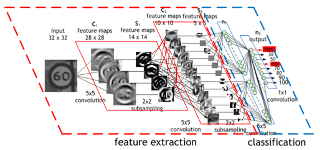
前面feature extraction部分体现了CNN的特点，feature extraction部分最后的输出可以作为分类器的输入。这个分类器你可以用softmax或RBF等等。

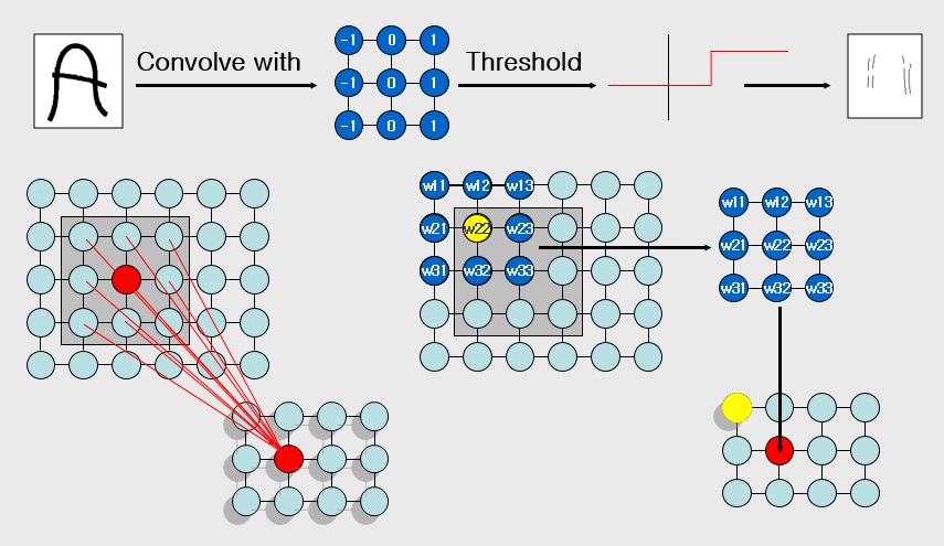
局部感受野与权值共享

权值共享指每一个map都由一个卷积核去做卷积得到。

权值共享减少了权值数量，降低了网络复杂度。

Conv layer

第一个卷积层对原输入图像进行卷积，后面的是对前一个卷积-采样层的S层的输出map进行卷积。

假设层为s层特征图像X_i^l-1（pooling层），l层为卷积C层，卷积结果为X_j^l

                 

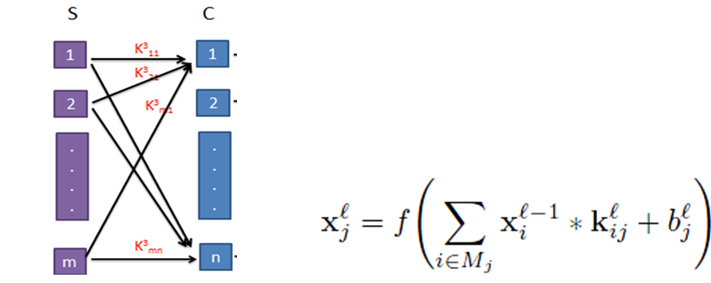
参数kij为两层间卷积核（滤波器，kernals），由于s层有m个特征，c层有n个特征，所以一共有m*n个卷积核。bj为卷基层每个结果特征对应的一个偏置项bias，f为非线性变换函数sigmoid函数；Mj为选择s层特征输入的个数，即选择多少个s层的图像特征作为输入；由于选择s层的特征个数方法不同，主要分为三种卷积选择方式

1、全部选择：

s层的全部特征都作为输入， Mj=m。如上图所示。

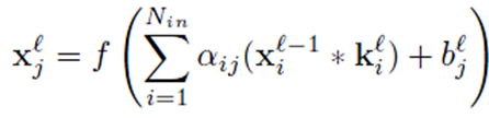
2、自动稀疏选择：

在卷积计算前加入稀疏稀疏aij，通过稀疏规则限制（论文后面），使算法自动选取部分s层特征作为输入，具体个数不确定。

3、部分选择：

按照一定的规则，固定的选取2个或者3个作为输入。

Subsampling  layer

下采样降低feature map的空间分辨率，从而实现一定程度的shift 和 distortion invariance。利用图像局部相关性的原理，对图像进行子抽样，可以减少数据处理量同时保留有用信息。这个过程也被称为pooling，常用pooling 有两种：

mean-pooling、max-pooling。

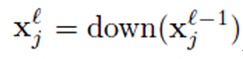
down(X_j^l-1)表示下采样操作，就是对一个小区域进行pooling操作，使数据降维。

有的算法还会对mean-pooling、max-pooling后的输出进行非线性映射

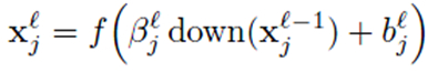
f可以是sigmoid函数。

输出层

最后一个卷积-采样层的输出可作为输出层的输入，输出层是全连接层，可采用svm、bp算法、softmax等分类算法。

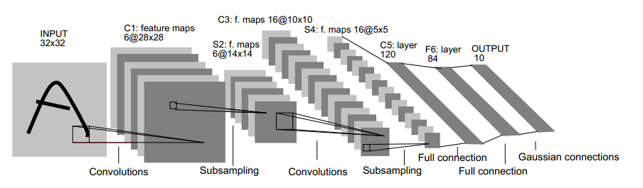
以LeNet5为例，其结构如下：

C1,C3,C5 : Convolutional layer. 
                 5 × 5 Convolution matrix.
S2 , S4 :    Subsampling layer.
                 Subsampling by factor 2.
F6 :           Fully connected layer

OUTPUT :  RBF

C层和S层成对出现，C承担特征抽取，S承担抗变形。C元中涉及两个重要参数，即感受野与阈值参数，前者确定输入连接的数目，后者则控制对特征子模式的反应程度。

C1层是一个卷积层（通过卷积运算，可以增强图像的某种特征，并且降低噪音），由6个特征图Feature Map构成。Feature Map中每个神经元与输入中5*5的邻域相连。特征图的大小为28*28。C1有156个可训练参数（每个滤波器5*5=25个unit参数和一个bias参数，一共6个滤波器，共(5*5+1)*6=156个参数），共156*(28*28)=122,304个连接。

S2层是一个下采样层，有6个14*14的特征图。特征图中的每个单元与C1中相对应特征图的2*2邻域相连接。S2层每个单元的4个输入相加，乘以一个可训练参数，再加上一个可训练偏置。结果通过sigmoid函数计算。可训练系数和偏置控制着sigmoid函数的非线性程度。如果系数比较小，那么运算近似于线性运算，亚采样相当于模糊图像。如果系数比较大，根据偏置的大小亚采样可以被看成是有噪声的“或”运算或者有噪声的“与”运算。每个单元的2*2感受野并不重叠，因此S2中每个特征图的大小是C1中特征图大小的1/4（行和列各1/2）。S2层有12个可训练参数和5880个连接。

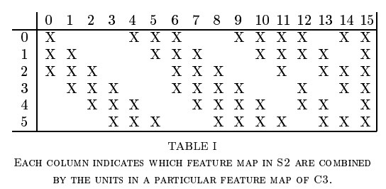
C3层也是一个卷积层，它同样通过5x5的卷积核去卷积层S2，然后得到的特征map就只有10x10个神经元，但是它有16种不同的卷积核，所以就存在16个特征map了。这里需要注意的一点是：C3中的每个特征map是连接到S2中的所有6个或者几个特征map的，表示本层的特征map是上一层提取到的特征map的不同组合。

S4层是一个下采样层，由16个5*5大小的特征图构成。特征图中的每个单元与C3中相应特征图的2*2邻域相连接，跟C1和S2之间的连接一样。S4层有32个可训练参数（每个特征图1个因子和一个偏置）和2000个连接。

C5层是一个卷积层，有120个特征图。每个单元与S4层的全部16个单元的5*5邻域相连。由于S4层特征图的大小也为5*5（同滤波器一样），故C5特征图的大小为1*1：这构成了S4和C5之间的全连接。之所以仍将C5标示为卷积层而非全相联层，是因为如果LeNet-5的输入变大，而其他的保持不变，那么此时特征图的维数就会比1*1大。C5层有48120个可训练连接。
F6层有84个单元（之所以选这个数字的原因来自于输出层的设计），与C5层全相连。有10164个可训练参数。如同经典神经网络，F6层计算输入向量和权重向量之间的点积，再加上一个偏置。然后将其传递给sigmoid函数产生单元i的一个状态。
最后，输出层由欧式径向基函数（Euclidean Radial Basis Function）单元组成，每类一个单元，每个有84个输入。换句话说，每个输出RBF单元计算输入向量和参数向量之间的欧式距离。输入离参数向量越远，RBF输出的越大。一个RBF输出可以被理解为衡量输入模式和与RBF相关联类的一个模型的匹配程度的惩罚项。用概率术语来说，RBF输出可以被理解为F6层配置空间的高斯分布的负log-likelihood。给定一个输入模式，损失函数应能使得F6的配置与RBF参数向量（即模式的期望分类）足够接近。这些单元的参数是人工选取并保持固定的（至少初始时候如此）。这些参数向量的成分被设为-1或1。虽然这些参数可以以-1和1等概率的方式任选，或者构成一个纠错码，但是被设计成一个相应字符类的7*12大小（即84）的格式化图片。

卷积核和偏置的初始化

卷积核和偏置在开始时要随机初始化，这些参数是要在训练过程中学习的。

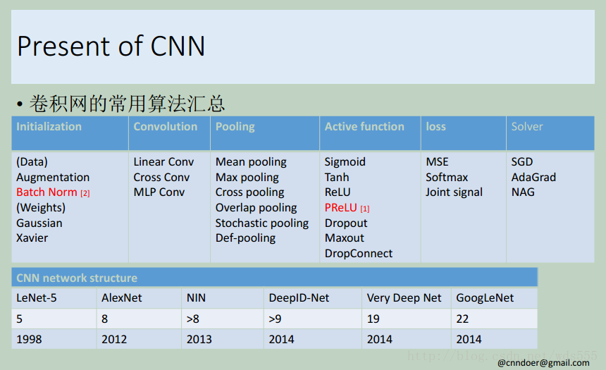
CNN涉及的算法

这张图来自博客http://blog.csdn.net/wds555/article/details/44100581，总结得很好

CNN网络算法流程

/*********** 训练阶段************/

/*********************************/

for t = 0; t < repeat; t++) 

{
epochsNum = trainset.size() / batchSize;

   for i = 0; i < epochsNum; i++

       {

          随机抽取batchSize个[0,size)的数batch[batchSize]作为本次批量训练的训练集    //size为总体trainSet的大小

           for j=0;j<batchSize;j++

               {

                  train(trainset.getRecord(batch[j]))

               }

         跑完一个batch后更新权重updateParas();

        }

       动态调整准学习速率

}

训练单个样本

train(Record record) {
forward(record);
boolean result = backPropagation(record);
return result;
}

反向传输
*/
private boolean backPropagation(Record record) {
boolean result = setOutLayerErrors(record);
setHiddenLayerErrors();
return result;
}

[python]  view plain copy

1. """This tutorial introduces the LeNet5 neural network architecture 
2. using Theano.  LeNet5 is a convolutional neural network, good for 
3. classifying images. This tutorial shows how to build the architecture, 
4. and comes with all the hyper-parameters you need to reproduce the 
5. paper's MNIST results. 
6. This implementation simplifies the model in the following ways: 
7.  - LeNetConvPool doesn't implement location-specific gain and bias parameters 
8.  - LeNetConvPool doesn't implement pooling by average, it implements pooling 
9.    by max. 
10.  - Digit classification is implemented with a logistic regression rather than 
11.    an RBF network 
12.  - LeNet5 was not fully-connected convolutions at second layer 
13. References: 
14.  - Y. LeCun, L. Bottou, Y. Bengio and P. Haffner: 
15.    Gradient-Based Learning Applied to Document 
16.    Recognition, Proceedings of the IEEE, 86(11):2278-2324, November 1998. 
17.    http://yann.lecun.com/exdb/publis/pdf/lecun-98.pdf 
18. """  
19. import os  
20. import sys  
21. import time  
22.   
23. import numpy  
24.   
25. import theano  
26. import theano.tensor as T  
27. from theano.tensor.signal import downsample  
28. from theano.tensor.nnet import conv  
29.   
30. from logistic_sgd import LogisticRegression, load_data  
31. from mlp import HiddenLayer  
32.   
33.   
34. class LeNetConvPoolLayer(object):  
35.     """Pool Layer of a convolutional network """  
36.   
37.     def __init__(self, rng, input, filter_shape, image_shape, poolsize=(2, 2)):  
38.         """ 
39.         Allocate a LeNetConvPoolLayer with shared variable internal parameters. 
40.         :type rng: numpy.random.RandomState 
41.         :param rng: a random number generator used to initialize weights 
42.         :type input: theano.tensor.dtensor4 
43.         :param input: symbolic image tensor, of shape image_shape 
44.         :type filter_shape: tuple or list of length 4 
45.         :param filter_shape: (number of filters, num input feature maps, 
46.                               filter height, filter width) 
47.         :type image_shape: tuple or list of length 4 
48.         :param image_shape: (batch size, num input feature maps, 
49.                              image height, image width) 
50.         :type poolsize: tuple or list of length 2 
51.         :param poolsize: the downsampling (pooling) factor (#rows, #cols) 
52.         """  
53.   
54.         assert image_shape[1] == filter_shape[1]  
55.         self.input = input  
56.   
57.         # there are "num input feature maps * filter height * filter width"  
58.         # inputs to each hidden unit  
59.         fan_in = numpy.prod(filter_shape[1:])  
60.         # each unit in the lower layer receives a gradient from:  
61.         # "num output feature maps * filter height * filter width" /  
62.         #   pooling size  
63.         fan_out = (filter_shape[0] * numpy.prod(filter_shape[2:]) /  
64.                    numpy.prod(poolsize))  
65.         # initialize weights with random weights  
66.         W_bound = numpy.sqrt(6. / (fan_in + fan_out))  
67.         self.W = theano.shared(  
68.             numpy.asarray(  
69.                 rng.uniform(low=-W_bound, high=W_bound, size=filter_shape),  
70.                 dtype=theano.config.floatX  
71.             ),  
72.             borrow=True  
73.         )  
74.   
75.         # the bias is a 1D tensor -- one bias per output feature map  
76.         b_values = numpy.zeros((filter_shape[0],), dtype=theano.config.floatX)  
77.         self.b = theano.shared(value=b_values, borrow=True)  
78.   
79.         # convolve input feature maps with filters  
80.         conv_out = conv.conv2d(  
81.             input=input,  
82.             filters=self.W,  
83.             filter_shape=filter_shape,  
84.             image_shape=image_shape  
85.         )  
86.   
87.         # downsample each feature map individually, using maxpooling  
88.         pooled_out = downsample.max_pool_2d(  
89.             input=conv_out,  
90.             ds=poolsize,  
91.             ignore_border=True  
92.         )  
93.   
94.         # add the bias term. Since the bias is a vector (1D array), we first  
95.         # reshape it to a tensor of shape (1, n_filters, 1, 1). Each bias will  
96.         # thus be broadcasted across mini-batches and feature map  
97.         # width & height  
98.         self.output = T.tanh(pooled_out + self.b.dimshuffle('x', 0, 'x', 'x'))  
99.   
100.         # store parameters of this layer  
101.         self.params = [self.W, self.b]  
102.   
103.   
104. def evaluate_lenet5(learning_rate=0.1, n_epochs=200,  
105.                     dataset='mnist.pkl.gz',  
106.                     nkerns=[20, 50], batch_size=500):  
107.     """ Demonstrates lenet on MNIST dataset 
108.     :type learning_rate: float 
109.     :param learning_rate: learning rate used (factor for the stochastic 
110.                           gradient) 
111.     :type n_epochs: int 
112.     :param n_epochs: maximal number of epochs to run the optimizer 
113.     :type dataset: string 
114.     :param dataset: path to the dataset used for training /testing (MNIST here) 
115.     :type nkerns: list of ints 
116.     :param nkerns: number of kernels on each layer 
117.     """  
118.   
119.     rng = numpy.random.RandomState(23455)  
120.   
121.     datasets = load_data(dataset)  
122.   
123.     train_set_x, train_set_y = datasets[0]  
124.     valid_set_x, valid_set_y = datasets[1]  
125.     test_set_x, test_set_y = datasets[2]  
126.   
127.     # compute number of minibatches for training, validation and testing  
128.     n_train_batches = train_set_x.get_value(borrow=True).shape[0]  
129.     n_valid_batches = valid_set_x.get_value(borrow=True).shape[0]  
130.     n_test_batches = test_set_x.get_value(borrow=True).shape[0]  
131.     n_train_batches /= batch_size  
132.     n_valid_batches /= batch_size  
133.     n_test_batches /= batch_size  
134.   
135.     # allocate symbolic variables for the data  
136.     index = T.lscalar()  # index to a [mini]batch  
137.   
138.     # start-snippet-1  
139.     x = T.matrix('x')   # the data is presented as rasterized images  
140.     y = T.ivector('y')  # the labels are presented as 1D vector of  
141.                         # [int] labels  
142.   
143.     ######################  
144.     # BUILD ACTUAL MODEL #  
145.     ######################  
146.     print '... building the model'  
147.   
148.     # Reshape matrix of rasterized images of shape (batch_size, 28 * 28)  
149.     # to a 4D tensor, compatible with our LeNetConvPoolLayer  
150.     # (28, 28) is the size of MNIST images.  
151.     layer0_input = x.reshape((batch_size, 1, 28, 28))  
152.   
153.     # Construct the first convolutional pooling layer:  
154.     # filtering reduces the image size to (28-5+1 , 28-5+1) = (24, 24)  
155.     # maxpooling reduces this further to (24/2, 24/2) = (12, 12)  
156.     # 4D output tensor is thus of shape (batch_size, nkerns[0], 12, 12)  
157.     layer0 = LeNetConvPoolLayer(  
158.         rng,  
159.         input=layer0_input,  
160.         image_shape=(batch_size, 1, 28, 28),  
161.         filter_shape=(nkerns[0], 1, 5, 5),  
162.         poolsize=(2, 2)  
163.     )  
164.   
165.     # Construct the second convolutional pooling layer  
166.     # filtering reduces the image size to (12-5+1, 12-5+1) = (8, 8)  
167.     # maxpooling reduces this further to (8/2, 8/2) = (4, 4)  
168.     # 4D output tensor is thus of shape (batch_size, nkerns[1], 4, 4)  
169.     layer1 = LeNetConvPoolLayer(  
170.         rng,  
171.         input=layer0.output,  
172.         image_shape=(batch_size, nkerns[0], 12, 12),  
173.         filter_shape=(nkerns[1], nkerns[0], 5, 5),  
174.         poolsize=(2, 2)  
175.     )  
176.   
177.     # the HiddenLayer being fully-connected, it operates on 2D matrices of  
178.     # shape (batch_size, num_pixels) (i.e matrix of rasterized images).  
179.     # This will generate a matrix of shape (batch_size, nkerns[1] * 4 * 4),  
180.     # or (500, 50 * 4 * 4) = (500, 800) with the default values.  
181.     layer2_input = layer1.output.flatten(2)  
182.   
183.     # construct a fully-connected sigmoidal layer  
184.     layer2 = HiddenLayer(  
185.         rng,  
186.         input=layer2_input,  
187.         n_in=nkerns[1] * 4 * 4,  
188.         n_out=500,  
189.         activation=T.tanh  
190.     )  
191.   
192.     # classify the values of the fully-connected sigmoidal layer  
193.     layer3 = LogisticRegression(input=layer2.output, n_in=500, n_out=10)  
194.   
195.     # the cost we minimize during training is the NLL of the model  
196.     cost = layer3.negative_log_likelihood(y)  
197.   
198.     # create a function to compute the mistakes that are made by the model  
199.     test_model = theano.function(  
200.         [index],  
201.         layer3.errors(y),  
202.         givens={  
203.             x: test_set_x[index * batch_size: (index + 1) * batch_size],  
204.             y: test_set_y[index * batch_size: (index + 1) * batch_size]  
205.         }  
206.     )  
207.   
208.     validate_model = theano.function(  
209.         [index],  
210.         layer3.errors(y),  
211.         givens={  
212.             x: valid_set_x[index * batch_size: (index + 1) * batch_size],  
213.             y: valid_set_y[index * batch_size: (index + 1) * batch_size]  
214.         }  
215.     )  
216.   
217.     # create a list of all model parameters to be fit by gradient descent  
218.     params = layer3.params + layer2.params + layer1.params + layer0.params  
219.   
220.     # create a list of gradients for all model parameters  
221.     grads = T.grad(cost, params)  
222.   
223.     # train_model is a function that updates the model parameters by  
224.     # SGD Since this model has many parameters, it would be tedious to  
225.     # manually create an update rule for each model parameter. We thus  
226.     # create the updates list by automatically looping over all  
227.     # (params[i], grads[i]) pairs.  
228.     updates = [  
229.         (param_i, param_i - learning_rate * grad_i)  
230.         for param_i, grad_i in zip(params, grads)  
231.     ]  
232.   
233.     train_model = theano.function(  
234.         [index],  
235.         cost,  
236.         updates=updates,  
237.         givens={  
238.             x: train_set_x[index * batch_size: (index + 1) * batch_size],  
239.             y: train_set_y[index * batch_size: (index + 1) * batch_size]  
240.         }  
241.     )  
242.     # end-snippet-1  
243.   
244.     ###############  
245.     # TRAIN MODEL #  
246.     ###############  
247.     print '... training'  
248.     # early-stopping parameters  
249.     patience = 10000  # look as this many examples regardless  
250.     patience_increase = 2  # wait this much longer when a new best is  
251.                            # found  
252.     improvement_threshold = 0.995  # a relative improvement of this much is  
253.                                    # considered significant  
254.     validation_frequency = min(n_train_batches, patience / 2)  
255.                                   # go through this many  
256.                                   # minibatche before checking the network  
257.                                   # on the validation set; in this case we  
258.                                   # check every epoch  
259.   
260.     best_validation_loss = numpy.inf  
261.     best_iter = 0  
262.     test_score = 0.  
263.     start_time = time.clock()  
264.   
265.     epoch = 0  
266.     done_looping = False  
267.   
268.     while (epoch < n_epochs) and (not done_looping):  
269.         epoch = epoch + 1  
270.         for minibatch_index in xrange(n_train_batches):  
271.   
272.             iter = (epoch - 1) * n_train_batches + minibatch_index  
273.   
274.             if iter % 100 == 0:  
275.                 print 'training @ iter = ', iter  
276.             cost_ij = train_model(minibatch_index)  
277.   
278.             if (iter + 1) % validation_frequency == 0:  
279.   
280.                 # compute zero-one loss on validation set  
281.                 validation_losses = [validate_model(i) for i  
282.                                      in xrange(n_valid_batches)]  
283.                 this_validation_loss = numpy.mean(validation_losses)  
284.                 print('epoch %i, minibatch %i/%i, validation error %f %%' %  
285.                       (epoch, minibatch_index + 1, n_train_batches,  
286.                        this_validation_loss * 100.))  
287.   
288.                 # if we got the best validation score until now  
289.                 if this_validation_loss < best_validation_loss:  
290.   
291.                     #improve patience if loss improvement is good enough  
292.                     if this_validation_loss < best_validation_loss *  \  
293.                        improvement_threshold:  
294.                         patience = max(patience, iter * patience_increase)  
295.   
296.                     # save best validation score and iteration number  
297.                     best_validation_loss = this_validation_loss  
298.                     best_iter = iter  
299.   
300.                     # test it on the test set  
301.                     test_losses = [  
302.                         test_model(i)  
303.                         for i in xrange(n_test_batches)  
304.                     ]  
305.                     test_score = numpy.mean(test_losses)  
306.                     print(('     epoch %i, minibatch %i/%i, test error of '  
307.                            'best model %f %%') %  
308.                           (epoch, minibatch_index + 1, n_train_batches,  
309.                            test_score * 100.))  
310.   
311.             if patience <= iter:  
312.                 done_looping = True  
313.                 break  
314.   
315.     end_time = time.clock()  
316.     print('Optimization complete.')  
317.     print('Best validation score of %f %% obtained at iteration %i, '  
318.           'with test performance %f %%' %  
319.           (best_validation_loss * 100., best_iter + 1, test_score * 100.))  
320.     print >> sys.stderr, ('The code for file ' +  
321.                           os.path.split(__file__)[1] +  
322.                           ' ran for %.2fm' % ((end_time - start_time) / 60.))  
323.   
324. if __name__ == '__main__':  
325.     evaluate_lenet5()  
326.   
327.   
328. def experiment(state, channel):  
329.     evaluate_lenet5(state.learning_rate, dataset=state.dataset)