


Dataset
本文的数据集pga.csv包含了职业高尔夫球手的发球统计信息,包含两个属性:accuracy 和 distance。accuracy 精确度描述了命中球道( fairways hit)的比例,Distances 描述的是发球的平均距离。我们的目的是用距离来预测命中率。在高尔夫中,一个人发球越远,那么精度会越低。
- 对于很多机器学习算法来说,输入数据前会先进行一些预处理,比如规范化,因为当计算两个样本的距离时,当一个属性的取值很大,那么这个距离会偏向取值较大的那个属性。由于此处的精度是百分比,而距离是码数。用到的规范化方法是每个元素减去均值然后除以标准方差。
import pandas
import matplotlib.pyplot as plt
pga = pandas.read_csv("pga.csv")

# Normalize the data  DataFrame可以用{.属性名}来调用一列数据的方式,返回ndarray对象
pga.distance = (pga.distance - pga.distance.mean()) / pga.distance.std()
pga.accuracy = (pga.accuracy - pga.accuracy.mean()) / pga.accuracy.std()
print(pga.head())

plt.scatter(pga.distance, pga.accuracy)
plt.xlabel('normalized distance')
plt.ylabel('normalized accuracy')
plt.show()
'''
   distance  accuracy
0  0.314379 -0.707727
1  1.693777 -1.586669
2 -0.059695 -0.176699
3 -0.574047  0.372640
4  1.343083 -1.934584
'''
Linear Model
- 观察数据散点图,发现距离和精度呈现负相关。首先用基本的线性回归LinearRegression 来拟合数据:
from sklearn.linear_model import LinearRegression
import numpy as np

# We can add a dimension to an array by using np.newaxis
print("Shape of the series:", pga.distance.shape) #这是一个ndarray对象,但是列数未知,因此需要人为指定一个
print("Shape with newaxis:", pga.distance[:, np.newaxis].shape)
'''
Shape of the series: (197,)
Shape with newaxis: (197, 1)
<class 'numpy.ndarray'>
<class 'pandas.core.series.Series'>
'''
# The X variable in LinearRegression.fit() must have 2 dimensions
lm = LinearRegression()
lm.fit(pga.distance[:, np.newaxis], pga.accuracy)
theta1 = lm.coef_[0]- 更简单的方法:
# 前面之所以要添加一个维度,是因为此时属性只有一列,但是X要求的是矩阵形(DataFrame或者二维ndarray)式,因此只要pga[['distance']]将distance放在列表中,取出来的就是一个DataFrame对象而不是Series对象。
from sklearn.linear_model import LinearRegression
import numpy as np
lm = LinearRegression()
lm.fit(pga[['distance']],pga.accuracy)
theta1 = lm.coef_[0]
Cost Function, Introduction
- 上述线性回归利用了sklearn中的包去估计模型的参数,用的是最小二乘法。最小二乘法通过矩阵计算可以很有效的拟合线性模型,并且提供确切的参数值。但是当矩阵的太大,直接用矩阵运算是不现实的,这时候就需要用一些迭代的方法来求解参数的估计值。梯度下降就是常见的一种迭代算法。
# The cost function of a single variable linear model
def cost(theta0, theta1, x, y):
    # Initialize cost
    J = 0
    # The number of observations
    m = len(x)
    # Loop through each observation
    for i in range(m):
        # Compute the hypothesis
        h = theta1 * x[i] + theta0
        # Add to cost
        J += (h - y[i])**2
    # Average and normalize cost
    J /= (2*m)
    return J

# The cost for theta0=0 and theta1=1
print(cost(0, 1, pga.distance, pga.accuracy))

theta0 = 100
theta1s = np.linspace(-3,2,100)
costs = []
for theta1 in theta1s:
    costs.append(cost(theta0, theta1, pga.distance, pga.accuracy))

plt.plot(theta1s, costs)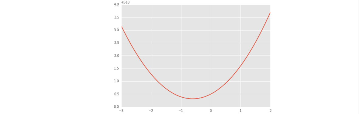
- 上面这段代码所做的工作是:将截距设置为100,系数设置为-3到2之间的100个等距离的值。然后计算每个系数所对应的模型的误差,误差公式如下,画出系数与误差的曲线图。发现在-0.7左右,模型的误差最小。

import numpy as np
from mpl_toolkits.mplot3d import Axes3D

theta0s = np.linspace(-2,2,100)
theta1s = np.linspace(-2,2, 100)
COST = np.empty(shape=(100,100))
# T0S:为100theta0s(theta1s的长度)行theta0s,T1S:为100列(theta0s的长度)theta1s
T0S, T1S = np.meshgrid(theta0s, theta1s)
# for each parameter combination compute the cost
for i in range(100):
    for j in range(100):
        COST[i,j] = cost(T0S[0,i], T1S[j,0], pga.distance, pga.accuracy)

# make 3d plot
fig2 = plt.figure()
ax = fig2.gca(projection='3d')
ax.plot_surface(X=T0S,Y=T1S,Z=COST)
plt.show()
上面这段代码首先用了一个新的函数meshgrid,参数为两个数组,第一个长度为m,第二个长度为n。因此返回的是第一个数组的n行复制,以及第二个数组的m列复制。举个例子:
x = [1,2,3],y=[5,6]————X=[[1,2,3],[1,2,3]],Y=[[5,5,5],[6,6,6]].然后去(X[i,j],Y[i,j])就可以得到x元素和y元素的任意组合。上述代码生成了一组系数,并且将误差与系数一起画了一个3D图。图中最低的地方就是最优解。
Cost Function, Slopes
1.本质相同:两种方法都是在给定已知数据(independent& dependent variables)的前提下对dependent variables算出出一个一般性的估值函数。然后对给定新数据的dependent variables进行估算。
2.目标相同:都是在已知数据的框架内,使得估算值与实际值的总平方差尽量更小(事实上未必一定要使用平方)。
3.实现方法和结果不同:最小二乘法是直接求导找出全局最小,是非迭代法。而梯度下降法是一种迭代法,先给定一个参数向量,然后向误差值下降最快的方向调整参数,在若干次迭代之后找到局部最小。梯度下降法的缺点是到最小点的时候收敛速度变慢,并且对初始点的选择极为敏感,其改进大多是在这两方面下功夫。当然, 其实梯度下降法还有别的其他用处, 比如其他找极值问题. 另外, 牛顿法也是一种不错的方法, 迭代收敛速度快于梯度下降法, 只是计算代价也比较高.
- 梯度下降法的步骤:初始化模型参数为w0,然后求误差关于每个参数的偏导,偏导的反方向就是下降最快的方向,因此将参数减去偏导的值,也可以加上学习率(下降的速度):
- 计算第一个参数theta0偏导:


# Partial derivative of cost in terms of theta0
def partial_cost_theta0(theta0, theta1, x, y):
    # Hypothesis
    h = theta0 + theta1*x
    # Difference between hypothesis and observation
    diff = (h - y)
    # Compute partial derivative
    partial = diff.sum() / (x.shape[0])
    return partial

partial0 = partial_cost_theta0(1, 1, pga.distance, pga.accuracy)
Gradient Descent Algorithm
- 从之前的可视化图中,可以从视觉上感受到,不同的斜率和截距将带来不同的误差,为了减少模型的误差,我们必须找到误差函数中参数的最优值。下面这段代码就是计算梯度下降的详细代码,一气呵成,结合了前面的函数,所以在完成一个大的工程时,预先写好一些小功能,然后在最后,拼接在一起就可以完成一个很好的功能:此处用到前面计算误差的函数cost(),以及计算偏导的函数partial_cost_theta0(),学会这种编程方式。
# x is our feature vector -- distance
# y is our target variable -- accuracy
# alpha is the learning rate
# theta0 is the intial theta0
# theta1 is the intial theta1
def gradient_descent(x, y, alpha=0.1, theta0=0, theta1=0):
    max_epochs = 1000 # Maximum number of iterations
    counter = 0      # Intialize a counter
    c = cost(theta1, theta0, pga.distance, pga.accuracy)  ## Initial cost
    costs = [c]     # Lets store each update
    # Set a convergence threshold to find where the cost function in minimized
    # When the difference between the previous cost and current cost
    #        is less than this value we will say the parameters converged
    convergence_thres = 0.000001
    cprev = c + 10
    theta0s = [theta0]
    theta1s = [theta1]

    # When the costs converge or we hit a large number of iterations will we stop updating
    while (np.abs(cprev - c) > convergence_thres) and (counter < max_epochs):
        cprev = c
        # Alpha times the partial deriviative is our updated
        update0 = alpha * partial_cost_theta0(theta0, theta1, x, y)
        update1 = alpha * partial_cost_theta1(theta0, theta1, x, y)

        # Update theta0 and theta1 at the same time
        # We want to compute the slopes at the same set of hypothesised parameters
        #             so we update after finding the partial derivatives
        theta0 -= update0
        theta1 -= update1

        # Store thetas
        theta0s.append(theta0)
        theta1s.append(theta1)

        # Compute the new cost
        c = cost(theta0, theta1, pga.distance, pga.accuracy)

        # Store updates
        costs.append(c)
        counter += 1   # Count

    return {'theta0': theta0, 'theta1': theta1, "costs": costs}

print("Theta1 =", gradient_descent(pga.distance, pga.accuracy)['theta1'])
descend = gradient_descent(pga.distance, pga.accuracy, alpha=.01)
plt.scatter(range(len(descend["costs"])), descend["costs"])
plt.show()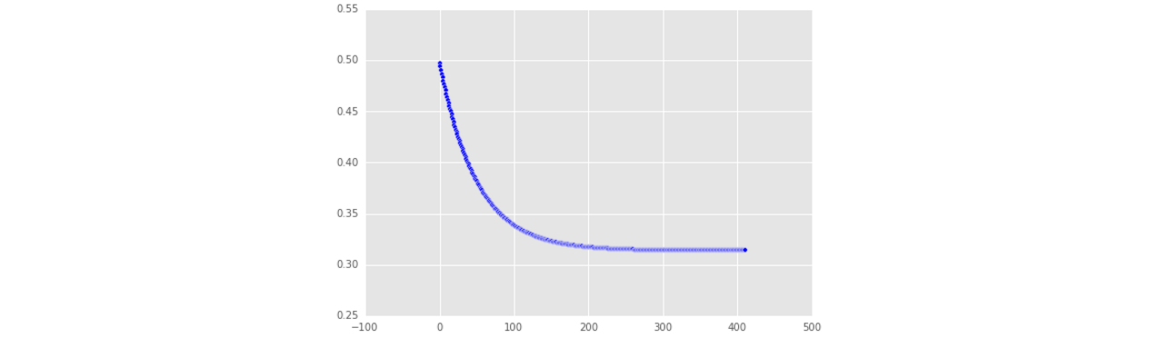


 2万+
2万+

 被折叠的 条评论
为什么被折叠?
被折叠的 条评论
为什么被折叠?
 到【灌水乐园】发言


