


上一篇文章我们介绍了causal attention和attention机制中的dropout,本文将继续介绍multi-head attention。
multi-head是指把attention机制分成多个head,每个head单独计算,每个head会关注当前单词与输入序列中其他单词在不同方面的上下文关系。上一篇文章中介绍的causal attention就可以看作是一个single-head attention。
multi-head,顾名思义,就是把多个single-head attention叠加起来。下面实现一个叠加多个CausalAttention类的multi-head attention:
class MultiHeadAttentionWrapper(nn.Module):

    def __init__(self, d_in, d_out, context_length, dropout, num_heads, qkv_bias=False):
        super().__init__()
        self.heads = nn.ModuleList(
            [CausalAttention(d_in, d_out, context_length, dropout, qkv_bias)
             for _ in range(num_heads)]
        )

    def forward(self, x):
        return torch.cat([head(x) for head in self.heads], dim=-1)


torch.manual_seed(123)

context_length = batch.shape[1] # This is the number of tokens
d_in, d_out = 3, 2
mha = MultiHeadAttentionWrapper(
    d_in, d_out, context_length, 0.0, num_heads=2
)

context_vecs = mha(batch)

print(context_vecs)
print("context_vecs.shape:", context_vecs.shape)
# 输出:
#tensor([[[-0.4519,  0.2216,  0.4772,  0.1063],
#         [-0.5874,  0.0058,  0.5891,  0.3257],
#         [-0.6300, -0.0632,  0.6202,  0.3860],
#         [-0.5675, -0.0843,  0.5478,  0.3589],
#         [-0.5526, -0.0981,  0.5321,  0.3428],
#         [-0.5299, -0.1081,  0.5077,  0.3493]],

#        [[-0.4519,  0.2216,  0.4772,  0.1063],
#         [-0.5874,  0.0058,  0.5891,  0.3257],
#         [-0.6300, -0.0632,  0.6202,  0.3860],
#         [-0.5675, -0.0843,  0.5478,  0.3589],
#         [-0.5526, -0.0981,  0.5321,  0.3428],
#         [-0.5299, -0.1081,  0.5077,  0.3493]]], grad_fn=<CatBackward0>)
# context_vecs.shape: torch.Size([2, 6, 4])
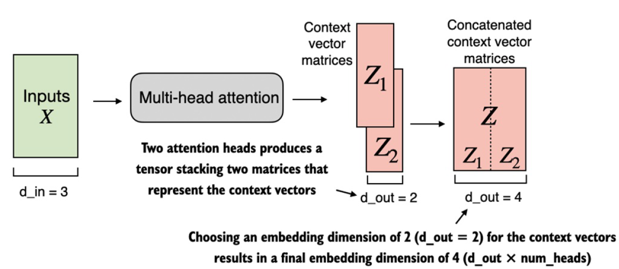
可以看到,输出结果的最后一个维度是4,而上一篇文章最后一个维度的输出是2,这是因为2个single-head attention的结果叠加(concat)起来了,示意图如下:
上面这种方法从功能上讲,完全可以实现multi-head attention的功能,但是每一个single-head都有自己的Wq, Wk, Wv权重矩阵,这不仅增加了参数量而且增加了计算量。下面介绍一种只有一套Wq, Wk, Wv权重矩阵的multi-head attention实现方法:
class MultiHeadAttention(nn.Module):
    def __init__(self, d_in, d_out, context_length, dropout, num_heads, qkv_bias=False):
        super().__init__()
        assert (d_out % num_heads == 0), \
            "d_out must be divisible by num_heads"

        self.d_out = d_out
        self.num_heads = num_heads
        self.head_dim = d_out // num_heads # Reduce the projection dim to match desired output dim

        self.W_query = nn.Linear(d_in, d_out, bias=qkv_bias)
        self.W_key = nn.Linear(d_in, d_out, bias=qkv_bias)
        self.W_value = nn.Linear(d_in, d_out, bias=qkv_bias)
        self.out_proj = nn.Linear(d_out, d_out)  # Linear layer to combine head outputs
        self.dropout = nn.Dropout(dropout)
        self.register_buffer(
            "mask",
            torch.triu(torch.ones(context_length, context_length),
                       diagonal=1)
        )

    def forward(self, x):
        b, num_tokens, d_in = x.shape
        # As in `CausalAttention`, for inputs where `num_tokens` exceeds `context_length`,
        # this will result in errors in the mask creation further below.
        # In practice, this is not a problem since the LLM (chapters 4-7) ensures that inputs
        # do not exceed `context_length` before reaching this forwar

        keys = self.W_key(x) # Shape: (b, num_tokens, d_out)
        queries = self.W_query(x)
        values = self.W_value(x)

        # We implicitly split the matrix by adding a `num_heads` dimension
        # Unroll last dim: (b, num_tokens, d_out) -> (b, num_tokens, num_heads, head_dim)
        keys = keys.view(b, num_tokens, self.num_heads, self.head_dim)
        values = values.view(b, num_tokens, self.num_heads, self.head_dim)
        queries = queries.view(b, num_tokens, self.num_heads, self.head_dim)

        # Transpose: (b, num_tokens, num_heads, head_dim) -> (b, num_heads, num_tokens, head_dim)
        keys = keys.transpose(1, 2)
        queries = queries.transpose(1, 2)
        values = values.transpose(1, 2)

        # Compute scaled dot-product attention (aka self-attention) with a causal mask
        attn_scores = queries @ keys.transpose(2, 3)  # Dot product for each head

        # Original mask truncated to the number of tokens and converted to boolean
        mask_bool = self.mask.bool()[:num_tokens, :num_tokens]

        # Use the mask to fill attention scores
        attn_scores.masked_fill_(mask_bool, -torch.inf)

        attn_weights = torch.softmax(attn_scores / keys.shape[-1]**0.5, dim=-1)
        attn_weights = self.dropout(attn_weights)

        # Shape: (b, num_tokens, num_heads, head_dim)
        context_vec = (attn_weights @ values).transpose(1, 2)

        # Combine heads, where self.d_out = self.num_heads * self.head_dim
        context_vec = context_vec.contiguous().view(b, num_tokens, self.d_out)
        context_vec = self.out_proj(context_vec) # optional projection

        return context_vec

torch.manual_seed(123)

batch_size, context_length, d_in = batch.shape
d_out = 2
mha = MultiHeadAttention(d_in, d_out, context_length, 0.0, num_heads=2)

context_vecs = mha(batch)

print(context_vecs)
print("context_vecs.shape:", context_vecs.shape)
# 输出:
#tensor([[[0.3190, 0.4858],
#         [0.2943, 0.3897],
#         [0.2856, 0.3593],
#         [0.2693, 0.3873],
#         [0.2639, 0.3928],
#         [0.2575, 0.4028]],

#        [[0.3190, 0.4858],
#         [0.2943, 0.3897],
#         [0.2856, 0.3593],
#         [0.2693, 0.3873],
#         [0.2639, 0.3928],
#         [0.2575, 0.4028]]], grad_fn=<ViewBackward0>)
# context_vecs.shape: torch.Size([2, 6, 2])
上面这中实现方法,只用了一套Wq, Wk, Wv,就实现了multi-head attention。其核心是将W权重矩阵分割成num_heads份,每一份单独计算,最后再合并。也就是说,上一种方法计算attention score时,每个单词向量的全部都参与计算,比如attention_scores(6×6) = queries(6×2) @ keys.T(2×6);第二种方法计算attention score时,每个单词向量被分割成了num_heads份,每个子份计算自己的attention score,即attention_scores(6×6) = queries(6×1) @ keys.T(1×6)。每个子份算出自己的上下文向量后再合并成总的上下文向量。
下面再以一个简单的例子,进一步理解上面例子中的多维矩阵的乘法:
# (b, num_heads, num_tokens, head_dim) = (1, 2, 3, 4)
a = torch.tensor([[[[0.2745, 0.6584, 0.2775, 0.8573],
                    [0.8993, 0.0390, 0.9268, 0.7388],
                    [0.7179, 0.7058, 0.9156, 0.4340]],

                   [[0.0772, 0.3565, 0.1479, 0.5331],
                    [0.4066, 0.2318, 0.4545, 0.9737],
                    [0.4606, 0.5159, 0.4220, 0.5786]]]])

print(a @ a.transpose(2, 3))
# 输出:
#tensor([[[[1.3208, 1.1631, 1.2879],
#          [1.1631, 2.2150, 1.8424],
#          [1.2879, 1.8424, 2.0402]],

#         [[0.4391, 0.7003, 0.5903],
#          [0.7003, 1.3737, 1.0620],
#          [0.5903, 1.0620, 0.9912]]]])
例子中a是一个四维矩阵,因此矩阵相乘会在最后2维(num_tokens, head_dim)上进行,然后每个head都会做一次矩阵相乘。下面对每个head进行分拆,分别单独计算:
first_head = a[0, 0, :, :]
first_res = first_head @ first_head.T
print("First head:\n", first_res)

second_head = a[0, 1, :, :]
second_res = second_head @ second_head.T
print("\nSecond head:\n", second_res)
# 输出:
# First head:
# tensor([[1.3208, 1.1631, 1.2879],
#        [1.1631, 2.2150, 1.8424],
#        [1.2879, 1.8424, 2.0402]])

# Second head:
# tensor([[0.4391, 0.7003, 0.5903],
#        [0.7003, 1.3737, 1.0620],
#        [0.5903, 1.0620, 0.9912]])
第二种方法MultiHeadAttention相比第一种方法MultiHeadAttentionWrapper,多了一些矩阵reshape和transpose的操作,更复杂但是更高效。因为我们只需要一套Wq, Wk, Wv计算queries, keys, values,分别只需要进行一次矩阵乘法(e.g. queries = self.W_query(x))。而在MultiHeadAttentionWrapper中,每个attention head都有一套Wq, Wk, Wv,都要重复进行矩阵乘法,而矩阵乘法是最耗资源的操作之一。因此第二种方法会更高效。
参考资料:
《Build a Large Language Model from Scratch》


 被折叠的 条评论
为什么被折叠?
被折叠的 条评论
为什么被折叠?
 到【灌水乐园】发言


