


引言
此文章为机器学习中线性回归的原理以及算法的代码实现,阅读之前需要具备机器学习概念,线性回归,梯度下降以及矩阵运算的基本知识。在本文中,会将机器学习中线性回归的数学基础理论和实现代码一并进行全面的讲解并展示算法及模型测评结果。
文中引用【这也太全了!回归算法、聚类算法、决策树、随机森林、神经网络、贝叶斯算法、支持向量机等十大机器学习算法一口气学完!-哔哩哔哩】的资料。
本文不作为商业用途,仅作记录供学习和回顾,若无意犯下错误,望及时指出,定第一时间改正。
理论基础
概念通俗解释
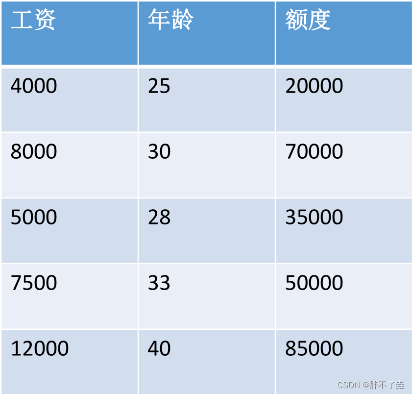
定义特征并给定数据与对应的标签,通过运算找到最合适的一条线(或一个面)来最好的拟合我们的数据点。
比如最简单的根据工资和年龄来预测银行会放予个人的贷款金额。
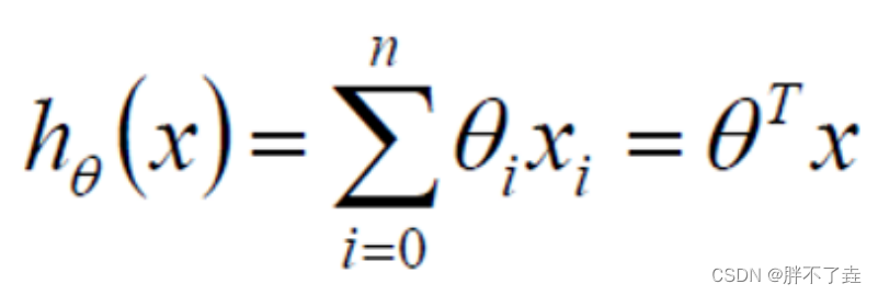
拟合的模型通式
![]()
在此式中,等号左边为预测的结果,右边是训练出的模型中的各个参数。theta1和theta2是各个特征在计算时的权重,theta0是拟合中的偏置值。体现在下图中即为theta1,theta2决定了坐标系中平面两条边的斜率,theta0决定了平面与y轴交点的高度。平面上的所有点为相应的x1,x2的预测结果。

由上述,我们可以推广到线性模型预测的通式,即
其中将对应的系数theta和相应的数据x的值作为矩阵进行计算,theta为一个n*1的矩阵,n为模型中的特征数量,x为一个数据行数*特征数的矩阵,即为数据集中值的矩阵。
误差
预测几乎不可能达到百分之百的拟合,真实值和预测值之间肯定是要存在差异的(用ε来表示该误差),因此在计算中引入误差是必要的。
对于每个样本都有下图公式,即预测值加上误差。
![]()
下面我们来对误差进行进一步的讲解,首先来看一个标准的解释
![]()
概念
误差是独立并且具有相同的分布,并且服从均值为0方差为theta^2的高斯分布(正态分布)
解释一下这个概念:
独立:任意两个特征之间不存在相互关系,即特征之间的取值互不干扰。
同分布:所有特征都应用在同一个目的同一个模型中。
由于误差服从高斯分布,所以有:(即为正态分布的p值)

通过上面的两个式子,我们可以推导得出

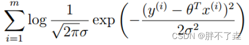
似然函数
组合后恰好是真实值的参数组成的函数
对于对数似然函数,当然是值越大和真实值越相近,拟合效果越好

对数似然
将乘法通过取对数转换成加法来计算

化简为
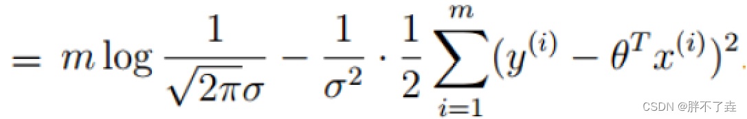
我们可以看到再1/2之前的量都为常量,简化为只看变量的式子
![]()
对于上述式子,要使得似然函数的值越大,就要令其值越小。
求偏导:

当偏导为0时取得最小值,即似然函数取得最大值,为我们训练的最终参数
![]()
评估
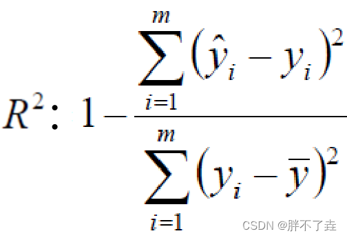
评估项R^2中,分子为残差平方和,分母为类似方差项。R^2越接近于1,模型拟合的越好。
梯度下降
机器学习顾名思义要有机器自主学习的过程,即认为定义一个方向,令其照这个方向进行训练。训练的过程要一步一步通过迭代优化参数完成。
原理
梯度下降即决定了参数优化更新的一系列指标,这里作简易解释,即每次优化后,参数的各项指标都会发生变化。梯度下降要确定参数每次改变时的变化率,可以当作斜率。还要确定每次变化率使用时参数变化的步长,步长可以理解为x轴值的变化量。步长确定,变化率确定,即可确定参数该如何进行调整,即可理解为y轴值的变化量。
梯度下降的核心在于确定了步长后,每一次更新后找到最快的参数优化变化率,从而能用最少的更新次数得到最优的参数组。这就是梯度下降的目的与简单原理。
目标函数:

批量梯度下降

用这个数据集的数据进行梯度下降,最稳健,但是时间成本较高。因此我们引入
随机梯度下降
![]()
由于只有一个样本,虽然迭代速度快,但不一定每次都朝着收敛的方向
综合考虑后最终形成
小批量梯度下降
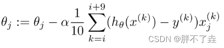
即每次取用一小部分数据,将上两种方式进行折中。
利用梯度下降,一步步完成对thetaj的更新迭代(α为步长),最终得到最优的模型参数组。
算法实现
以下是算法代码的目录
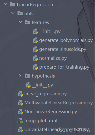
下面按逻辑顺序逐一讲解并展示
normalize.py
import numpy as np


def normalize(features):

    features_normalized = np.copy(features).astype(float)

    # 计算均值
    features_mean = np.mean(features, 0)

    # 计算标准差
    features_deviation = np.std(features, 0)

    # 标准化操作
    if features.shape[0] > 1:
        features_normalized -= features_mean

    # 防止除以0
    features_deviation[features_deviation == 0] = 1
    features_normalized /= features_deviation

    return features_normalized, features_mean, features_deviation
这是基本正则化的过程,代码较为简单,这里不过多讲解。其中输入的features为行是样本,列是特征的二维矩阵。输出为正则化后的矩阵,每个特征平均值组成的一维矩阵以及每个特征方差值组成的一维矩阵。
generate_sinusoids.py
import numpy as np


def generate_sinusoids(dataset, sinusoid_degree):
    """
    sin(x).
    """

    num_examples = dataset.shape[0]
    sinusoids = np.empty((num_examples, 0))

    for degree in range(1, sinusoid_degree + 1):
        sinusoid_features = np.sin(degree * dataset)
        sinusoids = np.concatenate((sinusoids, sinusoid_features), axis=1)

    return sinusoids
这是sin正则化的过程,代码较为简单,这里不过多讲解。其中输入的dataset为行是样本,列是特征的二维矩阵,sinusoid_degree为一个整数值,用来确定正则化程度。输出的sinusoids是和dataset形状相同,正则化后的矩阵。
generate_polynomials.py
import numpy as np
from .normalize import normalize


def generate_polynomials(dataset, polynomial_degree, normalize_data=False):
    """变换方法:
    x1, x2, x1^2, x2^2, x1*x2, x1*x2^2, etc.
    """

    features_split = np.array_split(dataset, 2, axis=1)
    dataset_1 = features_split[0]
    dataset_2 = features_split[1]

    (num_examples_1, num_features_1) = dataset_1.shape
    (num_examples_2, num_features_2) = dataset_2.shape

    if num_examples_1 != num_examples_2:
        raise ValueError('Can not generate polynomials for two sets with different number of rows')

    if num_features_1 == 0 and num_features_2 == 0:
        raise ValueError('Can not generate polynomials for two sets with no columns')

    if num_features_1 == 0:
        dataset_1 = dataset_2
    elif num_features_2 == 0:
        dataset_2 = dataset_1

    num_features = num_features_1 if num_features_1 < num_examples_2 else num_features_2
    dataset_1 = dataset_1[:, :num_features]
    dataset_2 = dataset_2[:, :num_features]

    polynomials = np.empty((num_examples_1, 0))

    for i in range(1, polynomial_degree + 1):
        for j in range(i + 1):
            polynomial_feature = (dataset_1 ** (i - j)) * (dataset_2 ** j)
            polynomials = np.concatenate((polynomials, polynomial_feature), axis=1)

    if normalize_data:
        polynomials = normalize(polynomials)[0]

    return polynomials
这是sin正则化的过程,代码较为简单,这里不过多讲解。其中输入的dataset为行是样本,列是特征的二维矩阵,polynomial_degree为一个整数值,用来确定正则化程度。输出的polynomials是和dataset形状相同,正则化后的矩阵。
在这里需要注意,执行完开头的矩阵split函数后,得到的是一个三维矩阵,因此在最后倒数第二行处,取索引[0]才是把正则化以后的矩阵取出。
prepare_for_training.py
import numpy as np
from .normalize import normalize
from .generate_sinusoids import generate_sinusoids
from .generate_polynomials import generate_polynomials


def prepare_for_training(data, polynomial_degree=0, sinusoid_degree=0, normalize_data=True):

    # 计算样本总数
    num_examples = data.shape[0]

    data_processed = np.copy(data)

    # 预处理
    features_mean = 0
    features_deviation = 0
    data_normalized = data_processed
    if normalize_data:
        (
            data_normalized,
            features_mean,
            features_deviation
        ) = normalize(data_processed)

        data_processed = data_normalized

    # 特征变换sinusoidal
    if sinusoid_degree > 0:
        sinusoids = generate_sinusoids(data_normalized, sinusoid_degree)
        data_processed = np.concatenate((data_processed, sinusoids), axis=1)

    # 特征变换polynomial
    if polynomial_degree > 0:
        polynomials = generate_polynomials(data_normalized, polynomial_degree, normalize_data)
        data_processed = np.concatenate((data_processed, polynomials), axis=1)

    # 加一列1
    data_processed = np.hstack((np.ones((num_examples, 1)), data_processed))

    return data_processed, features_mean, features_deviation
这是矩阵的预处理过程,具体为经上述三个正则化方式处理后再加一列1作为偏置值的初始值。
linear_regression.py
import numpy as np
from utils.features import prepare_for_training


class LinearRegression:

    def __init__(self,data,labels,polynomial_degree = 0,sinusoid_degree = 0,normalize_data=True):
        """
        1.对数据进行预处理操作
        2.先得到所有的特征个数
        3.初始化参数矩阵
        """
        (data_processed,
         features_mean,
         features_deviation) = prepare_for_training(data, polynomial_degree, sinusoid_degree,normalize_data=True)

        self.data = data_processed
        self.labels = labels
        self.features_mean = features_mean
        self.features_deviation = features_deviation
        self.polynomial_degree = polynomial_degree
        self.sinusoid_degree = sinusoid_degree
        self.normalize_data = normalize_data

        num_features = self.data.shape[1]
        self.theta = np.zeros((num_features,1))

    def train(self,alpha,num_iterations = 500):
        """
                    训练模块,执行梯度下降
        """
        cost_history = self.gradient_descent(alpha,num_iterations)
        return self.theta,cost_history

    def gradient_descent(self,alpha,num_iterations):
        """
                    实际迭代模块,会迭代num_iterations次
        """
        cost_history = []
        for _ in range(num_iterations):
            self.gradient_step(alpha)
            cost_history.append(self.cost_function(self.data,self.labels))
        return cost_history

    def gradient_step(self,alpha):
        """
                    梯度下降参数更新计算方法,注意是矩阵运算
        """
        num_examples = self.data.shape[0]
        prediction = LinearRegression.hypothesis(self.data,self.theta)
        delta = prediction - self.labels
        theta = self.theta
        theta = theta - alpha*(1/num_examples)*(np.dot(delta.T,self.data)).T
        self.theta = theta

    def cost_function(self,data,labels):
        """
                    损失计算方法
        """
        num_examples = data.shape[0]
        delta = LinearRegression.hypothesis(self.data,self.theta) - labels
        cost = (1/2)*np.dot(delta.T,delta)/num_examples
        return cost[0][0]

    @staticmethod
    def hypothesis(data,theta):
        predictions = np.dot(data,theta)
        return predictions

    def get_cost(self,data,labels):
        data_processed = prepare_for_training(data,
         self.polynomial_degree,
         self.sinusoid_degree,
         self.normalize_data
         )[0]

        return self.cost_function(data_processed,labels)
    def predict(self,data):
        """
                    用训练的参数模型,与预测得到回归值结果
        """
        data_processed = prepare_for_training(data,
         self.polynomial_degree,
         self.sinusoid_degree,
         self.normalize_data
         )[0]

        predictions = LinearRegression.hypothesis(data_processed,self.theta)

        return predictions
此类用作实例化模型,使用中直接实例化后调用train和predict方法即可。
UnivariateLinearRegression.py
import numpy as np
import pandas as pd
import matplotlib.pyplot as plt
from linear_regression import LinearRegression
data = pd.read_csv('../data/world-happiness-report-2017.csv')
# 得到训练和测试数据
train_data = data.sample(frac = 0.8)
test_data = data.drop(train_data.index)
input_param_name = 'Economy..GDP.per.Capita.'
output_param_name = 'Happiness.Score'
x_train = train_data[[input_param_name]].values
y_train = train_data[[output_param_name]].values
x_test = test_data[input_param_name].values
y_test = test_data[output_param_name].values
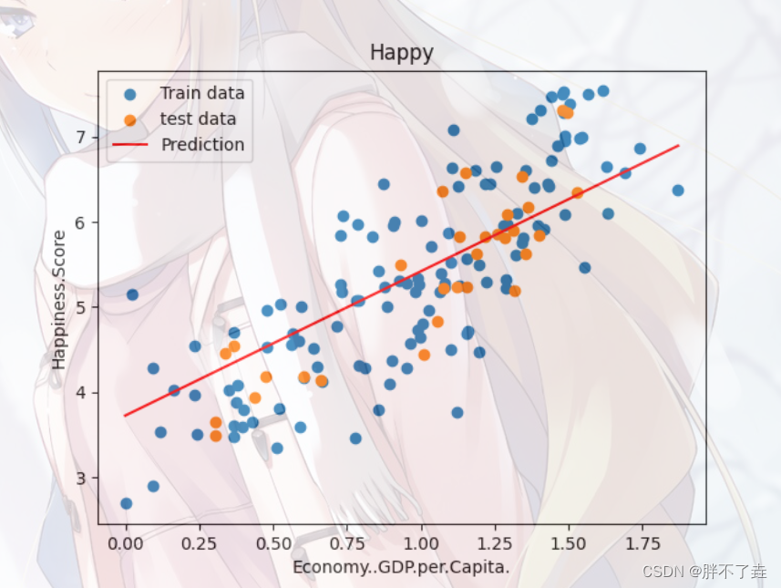
plt.scatter(x_train,y_train,label='Train data')
plt.scatter(x_test,y_test,label='test data')
plt.xlabel(input_param_name)
plt.ylabel(output_param_name)
plt.title('Happy')
plt.legend()
plt.show()
num_iterations = 500
learning_rate = 0.01
linear_regression = LinearRegression(x_train,y_train)
(theta,cost_history) = linear_regression.train(learning_rate,num_iterations)
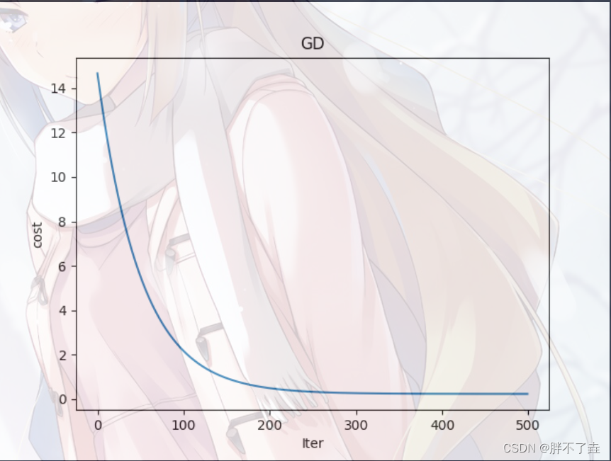
print ('开始时的损失:',cost_history[0])
print ('训练后的损失:',cost_history[-1])
plt.plot(range(num_iterations),cost_history)
plt.xlabel('Iter')
plt.ylabel('cost')
plt.title('GD')
plt.show()
predictions_num = 100
x_predictions = np.linspace(x_train.min(),x_train.max(),predictions_num).reshape(predictions_num,1)
y_predictions = linear_regression.predict(x_predictions)
plt.scatter(x_train,y_train,label='Train data')
plt.scatter(x_test,y_test,label='test data')
plt.plot(x_predictions,y_predictions,'r',label = 'Prediction')
plt.xlabel(input_param_name)
plt.ylabel(output_param_name)
plt.title('Happy')
plt.legend()
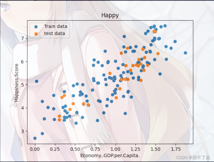
plt.show()这是预测单一特征的线性回归。
数据集自选并修改参数,但注意这是线性回归,数据应为连续的,不可用作分类。
预测结果如下形式

MultivariateLinearRegression.py
import numpy as np
import pandas as pd
import matplotlib.pyplot as plt
import plotly
import plotly.graph_objs as go

plotly.offline.init_notebook_mode()
from linear_regression import LinearRegression

data = pd.read_csv('../data/world-happiness-report-2017.csv')

train_data = data.sample(frac=0.8)
test_data = data.drop(train_data.index)

input_param_name_1 = 'Economy..GDP.per.Capita.'
input_param_name_2 = 'Freedom'
output_param_name = 'Happiness.Score'


x_train = train_data[[input_param_name_1, input_param_name_2]].values
y_train = train_data[[output_param_name]].values

x_test = test_data[[input_param_name_1, input_param_name_2]].values
y_test = test_data[[output_param_name]].values

# Configure the plot with training dataset.
plot_training_trace = go.Scatter3d(
    x=x_train[:, 0].flatten(),
    y=x_train[:, 1].flatten(),
    z=y_train.flatten(),
    name='Training Set',
    mode='markers',
    marker={
        'size': 10,
        'opacity': 1,
        'line': {
            'color': 'rgb(255, 255, 255)',
            'width': 1
        },
    }
)


plot_test_trace = go.Scatter3d(
    x=x_test[:, 0].flatten(),
    y=x_test[:, 1].flatten(),
    z=y_test.flatten(),
    name='Test Set',
    mode='markers',
    marker={
        'size': 10,
        'opacity': 1,
        'line': {
            'color': 'rgb(255, 255, 255)',
            'width': 1
        },
    }
)


plot_layout = go.Layout(
    title='Date Sets',
    scene={
        'xaxis': {'title': input_param_name_1},
        'yaxis': {'title': input_param_name_2},
        'zaxis': {'title': output_param_name}
    },
    margin={'l': 0, 'r': 0, 'b': 0, 't': 0}
)

plot_data = [plot_training_trace, plot_test_trace]

plot_figure = go.Figure(data=plot_data, layout=plot_layout)

plotly.offline.plot(plot_figure)

num_iterations = 500
learning_rate = 0.01
polynomial_degree = 0
sinusoid_degree = 0

linear_regression = LinearRegression(x_train, y_train, polynomial_degree, sinusoid_degree)

(theta, cost_history) = linear_regression.train(
    learning_rate,
    num_iterations
)

print('开始损失',cost_history[0])
print('结束损失',cost_history[-1])

plt.plot(range(num_iterations), cost_history)
plt.xlabel('Iterations')
plt.ylabel('Cost')
plt.title('Gradient Descent Progress')
plt.show()

predictions_num = 10

x_min = x_train[:, 0].min();
x_max = x_train[:, 0].max();

y_min = x_train[:, 1].min();
y_max = x_train[:, 1].max();


x_axis = np.linspace(x_min, x_max, predictions_num)
y_axis = np.linspace(y_min, y_max, predictions_num)


x_predictions = np.zeros((predictions_num * predictions_num, 1))
y_predictions = np.zeros((predictions_num * predictions_num, 1))

x_y_index = 0
for x_index, x_value in enumerate(x_axis):
    for y_index, y_value in enumerate(y_axis):
        x_predictions[x_y_index] = x_value
        y_predictions[x_y_index] = y_value
        x_y_index += 1

z_predictions = linear_regression.predict(np.hstack((x_predictions, y_predictions)))

plot_predictions_trace = go.Scatter3d(
    x=x_predictions.flatten(),
    y=y_predictions.flatten(),
    z=z_predictions.flatten(),
    name='Prediction Plane',
    mode='markers',
    marker={
        'size': 1,
    },
    opacity=0.8,
    surfaceaxis=2,
)

plot_data = [plot_training_trace, plot_test_trace, plot_predictions_trace]
plot_figure = go.Figure(data=plot_data, layout=plot_layout)
plotly.offline.plot(plot_figure)
预测结果如下形式


Non-linearRegression.py
import numpy as np
import pandas as pd
import matplotlib.pyplot as plt

from linear_regression import LinearRegression

data = pd.read_csv('../data/non-linear-regression-x-y.csv')

x = data['x'].values.reshape((data.shape[0], 1))
y = data['y'].values.reshape((data.shape[0], 1))

data.head(10)

plt.plot(x, y)
plt.show()

num_iterations = 50000
learning_rate = 0.02
polynomial_degree = 15
sinusoid_degree = 15
normalize_data = True

linear_regression = LinearRegression(x, y, polynomial_degree, sinusoid_degree, normalize_data)

(theta, cost_history) = linear_regression.train(
    learning_rate,
    num_iterations
)

print('开始损失: {:.2f}'.format(cost_history[0]))
print('结束损失: {:.2f}'.format(cost_history[-1]))

theta_table = pd.DataFrame({'Model Parameters': theta.flatten()})


plt.plot(range(num_iterations), cost_history)
plt.xlabel('Iterations')
plt.ylabel('Cost')
plt.title('Gradient Descent Progress')
plt.show()

predictions_num = 1000
x_predictions = np.linspace(x.min(), x.max(), predictions_num).reshape(predictions_num, 1);
y_predictions = linear_regression.predict(x_predictions)

plt.scatter(x, y, label='Training Dataset')
plt.plot(x_predictions, y_predictions, 'r', label='Prediction')
plt.show()
非线性数据可以预测,但是形式有限,仅预测这样的格式

features-_init_.py
from .normalize import normalize
from .generate_polynomials import generate_polynomials
from .generate_sinusoids import generate_sinusoids
from .prepare_for_training import prepare_for_training
仅初始化类。
其余文件
hypothesis类多余,无作用,可删除。
html文件是UnivariateLinearRegression.py执行后得到的三维图像。
结语
以上便是机器学习线性回归原理及代码实现的全部内容。文章体量不小,在写作中也许会出一些错误,欢迎大家指出,定第一时间改正。若代码或理论讲解不够详细,存在有问题也欢迎留言讨论。


 2万+
2万+


 被折叠的 条评论
为什么被折叠?
被折叠的 条评论
为什么被折叠?
 到【灌水乐园】发言


