tensorflow2------超参数搜索

1.超参数

超参数指的是：神经网络中有很多训练过程中不变化的参数，一般是在训练之前就已经认为设定好的，不像神经单元中权重与偏置都是在模型训练过程中值不断改变的。

• 网络结构参数：几层，每层宽度，每层激活函数等

• 训练参数：batch_size，学习率，学习率衰减算法等

(batch_size:指的是一次训练所选取的样本数。在没有使用Batch Size之前，这意味着网络在训练时，是一次把所有的数据（整个数据库）输入网络中，然后计算它们的梯度进行反向传播，由于在计算梯度时使用了整个数据库，所以计算得到的梯度方向更为准确。但是一旦在大型的数据库中一次性把所有数据输进网络，肯定会引起内存的爆炸。Batch Size的大小影响模型的优化程度和速度。同时其直接影响到GPU内存的使用情况，假如你GPU内存不大，该数值最好设置小一点。)

(学习率:指的是梯度下降时导数方向上前进的幅度；学习率衰减算法:学习率可以随着训练过程而变化，但是它有很多种不同变化的策略)

我们在训练过程中有很多的超参数，这些超参数组成了一个超参数集合。使用人力手工去设置尝试耗费时间且设置的参数不一定合适，所以这里使用了超参数搜索。

2.超参数搜索策略

超参数搜索策略分为以下四种：

网格搜索　随机搜索　遗传算法搜索　启发式搜索

1.网格搜索

所谓的网格搜索就是将各种超参数都离散化几个值，然后将这几个值一一组合起来，然后循环遍历这些超参数组合，尝试每一种可能性，表现最好的参数就是最终的结果，这种策略实际上就是暴力搜索而已，并不推荐使用。

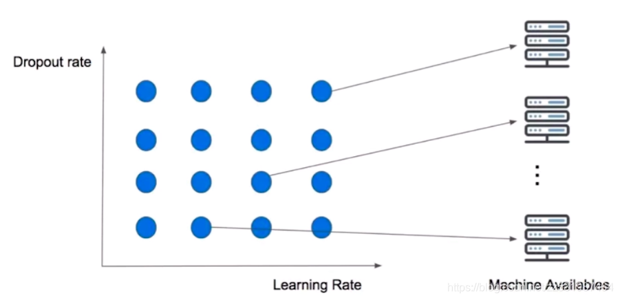
例如上面的就是将Dropout rate和Learning Rate相结合起来，定义一个n维方格，那么这里每格都对应一种超参数组合，总共就有16种不同的参数组合方法，然后循环遍历这16种不同的参数组合找到表现最好的参数组合，但是我们可以通过多台机器并行化的方式来缩短找到最优参数组合的时间。

2.随机搜索

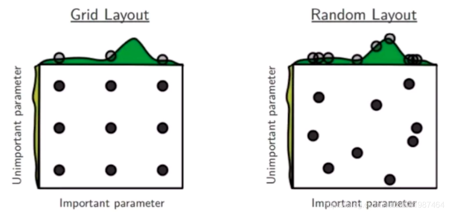
随机搜索相对于网格搜索其不同点在于：网格搜索只能取那些固定的参数组合，有可能会错过那样最优的参数组合；随机搜索是随机的取一些参数组合，这样最优解的参数组合是存在被取到的可能性，但是可能随机获取的参数组合可能会比较多。随机搜索一般用于粗选或普查。

3.遗传算法搜索

遗传算法（Genetic Algorithm）是一种通过模拟自然进化过程搜索最优解的方法，它的思想来自于进化论，生物种群具有自我进化的能力，能够不断适应环境，优势劣汰之后得到最优的种群个体。进化的行为主要有选择，遗传，变异，遗传算法希望能够通过将初始解空间进化到一个较好的解空间。

1. 初始化候选参数集合--->训练--->得到模型指标作为生存概率
2. 选择--->交叉--->变异--->产生下一代集合
3. 重新到1

详细的过程为：

我们首先初始化多组参数集合，然后对利用每一组参数进行训练得到模型的准确率，将模型的准确率指标作为生存概率，准确率高的生存概率就大；

然后我们选取准确率高的几组参数组合，交叉互换里面的参数形成新的参数组，然后对新的参数组里面的参数进行一些微小调整，从而这里便产生了新的参数集合；

产生了下一代的参数集合后我们重新回到第一步，继续利用新的参数组进行训练；

这样就能够较为准确地找到最优的参数组了。

4.启发式搜索(热点)

启发式搜索(Heuristically Search)又称为有信息搜索(Informed Search)，它是利用问题拥有的启发信息来引导搜索，达到减少搜索范围、降低问题复杂度的目的，这种利用启发信息的搜索过程称为启发式搜索。

原理：在状态空间中的搜索对每一个搜索的位置进行评估，得到最好的位置，再从这个位置进行搜索直到目标。这样可以省略大量无谓的搜索路径，提高了效率。在启发式搜索中，对位置的估价是十分重要的。采用了不同的估价可以有不同的效果。

启发式搜索有模拟退火算法(SA)、遗传算法(GA)、列表搜索算法(ST)、进化规划(EP)、进化策略(ES)、蚁群算法(ACA)、人工神经网络(ANN)...等。

• 研究热点---AutoML
• 使用循环神经网络来生成参数，不像前面的随机搜索一样随机生成参数组
• 使用前面生成的参数形成一个新的网络结构，然后在上面进行训练，训练完使用强化学习形成一个反馈机制，再反过来训练循环神经网络。。到最后，循环神经网络被训练好的时候，那它预测的网络结构就是最优的网络结构

上面就是启发式搜索的核心操作步骤。

3.接下来在代码中实现超参数搜索

1.该示例简单的使用遍历一个Learning_rate的数据集合来找到最优的学习率超参数

import matplotlib as mpl #画图用的库
import matplotlib.pyplot as plt
#下面这一句是为了可以在notebook中画图
%matplotlib inline
import numpy as np
import sklearn   #机器学习算法库
import pandas as pd #处理数据的库   
import os
import sys
import time
import tensorflow as tf

from tensorflow import keras   #使用tensorflow中的keras
#import keras #单纯的使用keras

print(tf.__version__)
print(sys.version_info)
for module in mpl, np, sklearn, pd, tf, keras:
    print(module.__name__, module.__version__)




2.0.0
sys.version_info(major=3, minor=6, micro=9, releaselevel='final', serial=0)
matplotlib 3.1.2
numpy 1.18.0
sklearn 0.21.3
pandas 0.25.3
tensorflow 2.0.0
tensorflow_core.keras 2.2.4-tf

#引用位于sklearn数据集中的房价预测数据集
from sklearn.datasets import fetch_california_housing

housing = fetch_california_housing()
print(housing.DESCR) #数据集的描述
print(housing.data.shape) #相当于 x
print(housing.target.shape) #相当于 y




.. _california_housing_dataset:

California Housing dataset
--------------------------

**Data Set Characteristics:**

    :Number of Instances: 20640

    :Number of Attributes: 8 numeric, predictive attributes and the target

    :Attribute Information:
        - MedInc        median income in block
        - HouseAge      median house age in block
        - AveRooms      average number of rooms
        - AveBedrms     average number of bedrooms
        - Population    block population
        - AveOccup      average house occupancy
        - Latitude      house block latitude
        - Longitude     house block longitude

    :Missing Attribute Values: None

This dataset was obtained from the StatLib repository.
http://lib.stat.cmu.edu/datasets/

The target variable is the median house value for California districts.

This dataset was derived from the 1990 U.S. census, using one row per census
block group. A block group is the smallest geographical unit for which the U.S.
Census Bureau publishes sample data (a block group typically has a population
of 600 to 3,000 people).

It can be downloaded/loaded using the
:func:`sklearn.datasets.fetch_california_housing` function.

.. topic:: References

    - Pace, R. Kelley and Ronald Barry, Sparse Spatial Autoregressions,
      Statistics and Probability Letters, 33 (1997) 291-297

(20640, 8)
(20640,)

#查看当前x、y的数据类型

import pprint #pprint()模块打印出来的数据结构更加完整,对于数据结构比较复杂、数据长度较长的数据，适合采用pprint()

pprint.pprint(housing.data[0:5])
pprint.pprint(housing.target[0:5])




array([[ 8.32520000e+00,  4.10000000e+01,  6.98412698e+00,
         1.02380952e+00,  3.22000000e+02,  2.55555556e+00,
         3.78800000e+01, -1.22230000e+02],
       [ 8.30140000e+00,  2.10000000e+01,  6.23813708e+00,
         9.71880492e-01,  2.40100000e+03,  2.10984183e+00,
         3.78600000e+01, -1.22220000e+02],
       [ 7.25740000e+00,  5.20000000e+01,  8.28813559e+00,
         1.07344633e+00,  4.96000000e+02,  2.80225989e+00,
         3.78500000e+01, -1.22240000e+02],
       [ 5.64310000e+00,  5.20000000e+01,  5.81735160e+00,
         1.07305936e+00,  5.58000000e+02,  2.54794521e+00,
         3.78500000e+01, -1.22250000e+02],
       [ 3.84620000e+00,  5.20000000e+01,  6.28185328e+00,
         1.08108108e+00,  5.65000000e+02,  2.18146718e+00,
         3.78500000e+01, -1.22250000e+02]])
array([4.526, 3.585, 3.521, 3.413, 3.422])

#用sklearn中专门用于划分训练集和测试集的方法
from sklearn.model_selection import train_test_split

#train_test_split默认将数据划分为3:1，我们可以通过修改test_size值来改变数据划分比例(默认0.25，即3:1)
#将总数乘以test_size就表示test测试集、valid验证集数量
#将数据集整体拆分为train_all和test数据集
x_train_all,x_test, y_train_all,y_test = train_test_split(housing.data, housing.target, random_state=7)
#将train_all数据集拆分为train训练集和valid验证集
x_train,x_valid, y_train,y_valid = train_test_split(x_train_all, y_train_all, random_state=11)

print(x_train_all.shape,y_train_all.shape)
print(x_test.shape, y_test.shape)
print(x_train.shape, y_train.shape)
print(x_valid.shape, y_valid.shape)




(15480, 8) (15480,)
(5160, 8) (5160,)
(11610, 8) (11610,)
(3870, 8) (3870,)

#训练数据归一化处理
# x = (x - u)/std  u为均值，std为方差
from sklearn.preprocessing import StandardScaler #使用sklearn中的StandardScaler实现训练数据归一化

scaler = StandardScaler()#初始化一个scaler对象
x_train_scaler = scaler.fit_transform(x_train)#x_train已经是二维数据了，无需astype转换
x_valid_scaler = scaler.transform(x_valid)
x_test_scaler  = scaler.transform(x_test)

#tf.keras.models.Sequential()建立模型
# 这里仅设置learning_rate: [1e-4, 3e-4, 1e-3, 3e-3, 1e-2, 3e-2]
# W = W + grad * learning_rate

learning_rates = [1e-4, 3e-4, 1e-3, 3e-3, 1e-2, 3e-2]
histories = []
for lr in learning_rates:
    
    model = keras.models.Sequential([
        keras.layers.Dense(30, activation="relu",input_shape=x_train.shape[1:]),
        keras.layers.Dense(1),
    ])
    
    #注：我们在训练迭代100次的过程中lr并不会发生变化，实际上我们可以使用 学习率衰减算法 来对lr进行动态调整
    optimizer = keras.optimizers.SGD(lr)
    
    
    #编译model。 loss目标函数为均方差，这里表面上是字符串，实际上tensorflow中会映射到对应的算法函数，我们也可以自定义
    model.compile(loss="mean_squared_error", optimizer=optimizer)#"adam")

    #使用监听模型训练过程中的callbacks
    logdir='./callbacks_regression'
    if not os.path.exists(logdir):
        os.mkdir(logdir)
    output_model_file = os.path.join(logdir,"regression_california_housing.h5")

    #首先定义一个callback数组
    callbacks = [
        keras.callbacks.TensorBoard(logdir),
        keras.callbacks.ModelCheckpoint(output_model_file,save_best_only=True),
        keras.callbacks.EarlyStopping(patience=5,min_delta=1e-3)
    ]    
    history=model.fit(x_train_scaler,y_train,epochs=100,
                     validation_data=(x_valid_scaler,y_valid),
                     callbacks=callbacks)
    histories.append(history)

#打印模型训练过程中的相关曲线
def plot_learning_curves(history):
    pd.DataFrame(history.history).plot(figsize=(8,5))
    plt.grid(True)
    plt.gca().set_ylim(0,1)
    plt.show()
    
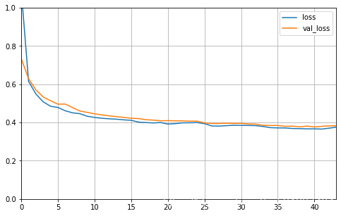
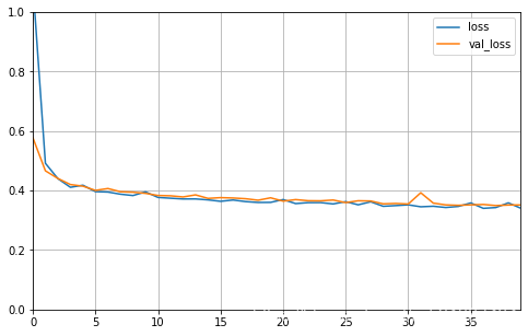
for lr, history in zip(learning_rates, histories):#并行遍历，lr遍历learning_rate， history遍历histories
    print("learning_rate:",lr)
    plot_learning_curves(history)

learning_rate: 0.0001

learning_rate: 0.0003

learning_rate: 0.001

learning_rate: 0.003

learning_rate: 0.01

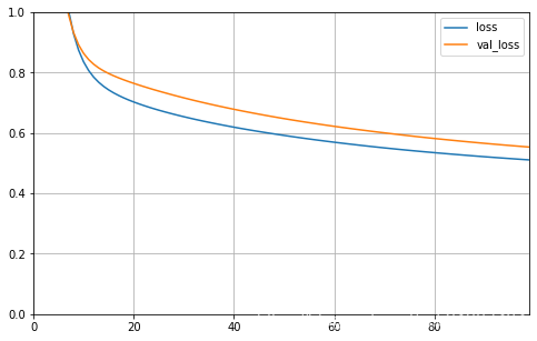
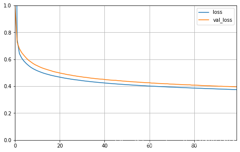
learning_rate: 0.03 #下图说明此时梯度已经爆炸了

从损失函数的曲线图中我们可以看到，在学习率为0.01时，其loss值最低，也就是说当超参数learning_rate为0.01时模型效果最优

 

2.sklearn超参数搜索

 这里有以下几个重点：

• 封装tf.keras中的model构建，封装成build_model
• 将tf.keras的model转换为 sklearn的model
• 定义参数集合
• 搜索参数

import matplotlib as mpl #画图用的库
import matplotlib.pyplot as plt
#下面这一句是为了可以在notebook中画图
%matplotlib inline
import numpy as np
import sklearn   #机器学习算法库
import pandas as pd #处理数据的库   
import os
import sys
import time
import tensorflow as tf

from tensorflow import keras   #使用tensorflow中的keras
#import keras #单纯的使用keras

print(tf.__version__)
print(sys.version_info)
for module in mpl, np, sklearn, pd, tf, keras:
    print(module.__name__, module.__version__)

#引用位于sklearn数据集中的房价预测数据集
from sklearn.datasets import fetch_california_housing

housing = fetch_california_housing()
print(housing.DESCR) #数据集的描述
print(housing.data.shape) #相当于 x
print(housing.target.shape) #相当于 y

#查看当前x、y的数据类型

import pprint #pprint()模块打印出来的数据结构更加完整,对于数据结构比较复杂、数据长度较长的数据，适合采用pprint()

pprint.pprint(housing.data[0:5])
pprint.pprint(housing.target[0:5])

#用sklearn中专门用于划分训练集和测试集的方法
from sklearn.model_selection import train_test_split

#train_test_split默认将数据划分为3:1，我们可以通过修改test_size值来改变数据划分比例(默认0.25，即3:1)
#将总数乘以test_size就表示test测试集、valid验证集数量
#将数据集整体拆分为train_all和test数据集
x_train_all,x_test, y_train_all,y_test = train_test_split(housing.data, housing.target, random_state=7)
#将train_all数据集拆分为train训练集和valid验证集
x_train,x_valid, y_train,y_valid = train_test_split(x_train_all, y_train_all, random_state=11)

print(x_train_all.shape,y_train_all.shape)
print(x_test.shape, y_test.shape)
print(x_train.shape, y_train.shape)
print(x_valid.shape, y_valid.shape)

#训练数据归一化处理
# x = (x - u)/std  u为均值，std为方差
from sklearn.preprocessing import StandardScaler #使用sklearn中的StandardScaler实现训练数据归一化

scaler = StandardScaler()#初始化一个scaler对象
x_train_scaler = scaler.fit_transform(x_train)#x_train已经是二维数据了，无需astype转换
x_valid_scaler = scaler.transform(x_valid)
x_test_scaler  = scaler.transform(x_test)

#使用sklearn中的RandomizedSearchCV实现超参数的随机化搜索
#1.首先需要tf.keras.models转换为sklearn形式的model
#2.定义参数集合
#3.使用RandomizedSearchCV去搜索参数

#这里主要将tf.keras的model定义 封装为一个 build_model模块
def build_model(hidden_layers=1,layers_size=30,learning_rate=3e-3):
    model=keras.models.Sequential()
    model.add(keras.layers.Dense(layers_size,activation='relu',input_shape=x_train.shape[1:]))
    
    #中间添加n个隐藏全连接层
    for _ in range(hidden_layers - 1):
        model.add(keras.layers.Dense(layers_size,activation='relu'))
    
    #添加输出层
    model.add(keras.layers.Dense(1))
    
    optimizer=keras.optimizers.SGD(learning_rate)
    model.compile(loss='mse',optimizer=optimizer)#mean_squared_error简写mse
    return model

#将tf.keras.model转换为 sklearn_model
sklearn_model=keras.wrappers.scikit_learn.KerasRegressor(build_model)

#使用监听模型训练过程中的callbacks
logdir='./callbacks_regression-hp-search'
import shutil
if os.path.exists(logdir):
    shutil.rmtree(logdir) #先强制删除该文件夹，后面再新建
else:
    os.mkdir(logdir)
output_model_file = os.path.join(logdir,"regression_california_housing-hp-search.h5")

#首先定义一个callback数组
callbacks = [
    keras.callbacks.TensorBoard(logdir),
    keras.callbacks.ModelCheckpoint(output_model_file,save_best_only=True),
    keras.callbacks.EarlyStopping(patience=5,min_delta=1e-3)
]

history = sklearn_model.fit(x_train_scaler,y_train,epochs=100,
                 validation_data=(x_valid_scaler,y_valid),callbacks=callbacks)

#打印模型训练过程中的相关曲线
def plot_learning_curves(history):
    pd.DataFrame(history.history).plot(figsize=(8,5))
    plt.grid(True)
    plt.gca().set_ylim(0,1)
    plt.show()
'''
for lr, history in zip(learning_rates, histories):#并行遍历，lr遍历learning_rate， history遍历histories
    print("learning_rate:",lr)
    plot_learning_curves(history)
'''
plot_learning_curves(history)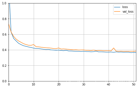

#model.evaluate(x_test_scaler,y_test)#sklearn中的model没有evaluate函数

from scipy.stats import reciprocal
#分布函数f(x) = 1/(x*log(b/a)) a <= x <= b

#在1e-4至1e-2之间取10个数，看下示例，注释运行
#reciprocal.rvs(1e-4,1e-2,size=10) 
#array([0.00194792, 0.0030323 , 0.00012433, 0.00113947, 0.00015001,
#       0.0085196 , 0.00514795, 0.00038299, 0.00644926, 0.00039257])

#定义一个参数分布，这个参数分布里面的参数(hidden_layers、layers_size、learning_rate)设置取决于前面封装的build_model接口参数
param_distribution={
    "hidden_layers":[1,2,3,4],
    #这里sklearn的版本必须是 0.21.3，不然下面的写法会报错
    "layers_size":np.arange(1, 40),#取值为 [1,2,3...98,99,100]
    "learning_rate":reciprocal(1e-4,1e-2),#lr是一个连续取值，使用分布来取learning_rate值
    
    #在最新版sklearn0.22.2版本中上面的搜索写法执行报错，只能用下面普通列表才不会报错，但是这样写实际上意义不是很大
    #"layers_size": [5, 10, 20, 30, 40, 50],
    #"learning_rate": [1e-4, 5e-5, 1e-3, 5e-3, 1e-2],    
}

from sklearn.model_selection import RandomizedSearchCV

#n_iter:从前面的参数分布中取出的参数组的个数; n_jobs:并行化处理的任务个数
random_search_cv=RandomizedSearchCV(sklearn_model,param_distribution,n_iter=10,n_jobs=1)
random_search_cv.fit(x_train_scaler,y_train,epochs=30,validation_data=(x_valid_scaler,y_valid),callbacks=callbacks)




Train on 7740 samples, validate on 3870 samples
Epoch 1/30
7740/7740 [==============================] - 1s 91us/sample - loss: 3.7549 - val_loss: 2.5928
Epoch 2/30
7740/7740 [==============================] - 0s 64us/sample - loss: 1.8982 - val_loss: 1.5324
Epoch 3/30
7740/7740 [==============================] - 0s 54us/sample - loss: 1.2397 - val_loss: 1.1008
。。。
RandomizedSearchCV(cv='warn', error_score='raise-deprecating',
                   estimator=<tensorflow.python.keras.wrappers.scikit_learn.KerasRegressor object at 0x7f01f9d40240>,
                   iid='warn', n_iter=10, n_jobs=1,
                   param_distributions={'hidden_layers': [1, 2, 3, 4],
                                        'layers_size': array([ 1,  2,  3,  4,  5,  6,  7,  8,  9, 10, 11, 12, 13, 14, 15, 16, 17,
       18, 19, 20, 21, 22, 23, 24, 25, 26, 27, 28, 29, 30, 31, 32, 33, 34,
       35, 36, 37, 38, 39]),
                                        'learning_rate': <scipy.stats._distn_infrastructure.rv_frozen object at 0x7f01f9ffcd68>},
                   pre_dispatch='2*n_jobs', random_state=None, refit=True,
                   return_train_score=False, scoring=None, verbose=0)

#打印最优的超参数的数据
print(random_search_cv.best_params_)
print(random_search_cv.best_score_)
print(random_search_cv.best_estimator_)



{'hidden_layers': 4, 'layers_size': 23, 'learning_rate': 0.00650462432478528}
-0.3407047720714236
<tensorflow.python.keras.wrappers.scikit_learn.KerasRegressor object at 0x7f01a415ceb8>

#获取最优超参数的模型并在测试集上验证下
model=random_search_cv.best_estimator_.model
model.evaluate(x_test_scaler,y_test)



5160/1 [==================。。。==================================================] - 0s 30us/sample - loss: 0.3822
0.3205111207426056