深度学习之四：卷积神经网络基础

最新推荐文章于 2024-07-07 22:33:07 发布

zzulp

最新推荐文章于 2024-07-07 22:33:07 发布

阅读量3.1k

点赞数

分类专栏： ML

本文链接：https://blog.csdn.net/zzulp/article/details/79337786

版权

ML 专栏收录该内容

15 篇文章 5 订阅

订阅专栏

计算机视觉在深度学习的帮助下取得了令人惊叹的进展，其中发挥重要作用的是卷积神经网络。本节总结了卷积神经的原理与实现方法。

1 卷积神经网络

1.1 计算机视觉与深度学习

计算机视觉要解决的问题是如何让机器理解现实世界的现象。目前主要处理的问题如图像分类，目标检测，风格变换等。

对于小型图片，如MNIST的图片处理，图像大小为64*64，使用全连接神经网络还可以处理。如果图像较大，如1000*1000*3时，单个输入层就需要3M的节点，全连接情况下，单层的权重就可能多达数十亿的待训练参数。这将导致神经网络无法进行有效训练。因此业界提出卷积神经网络解决参数过多的问题。

先看一个卷积神经网络的结构，在卷积神经网络中包括三种类型的层：卷积层，池化层和全连接层。下面几节介绍卷积神经网络的基本概念。
此处输入图片的描述

1.2 过滤器

在卷积神经网络中，过滤器也称为卷积核，通常是3*3或5*5的小型矩阵(先忽略每个点可能有多个通道)。过滤器的作用是和输入图像的各个区域逐次进行卷积。

所谓卷积运算是计算两个矩阵的对应元素(Element-wise)乘积的和。卷积本质是两个向量的内积，体现了两个向量的距离。

下图展示了过滤器在输入图像上的卷积计算的过程：
输入图像与过滤器的卷积计算过程

因此过滤器可以捕获图像中与之类似模式的图像区域。例如下图展示了一个过滤器的数值矩阵与图形。
此处输入图片的描述

当使用这个过滤器在图像上移动并计算卷积时，不同的区域会有不同的卷积结果。
此处输入图片的描述

在类似于的模式下过滤器与图像区域的卷积会产生较大的值。
此处输入图片的描述
不相似的区域则产生较小的值。

此外在一层上捕获的模式可以组合为更复杂的模式并输入到下一层，从而使得下一层能识别更复杂的图像模式。

训练CNN在一定意义上是在训练每个卷积层的过滤器，让其组合对特定的模式有高的激活，以达到CNN网络的分类/检测等目的。

1.3 Padding

对于一个shape为 $[n,n]$ 的图像，若过滤器的 shape为 $[f,f]$ ，在卷积时每次移动1步，则生成的矩阵shape为 $[n-f+1, n-f+1]$ 。这样如果经过多层的卷积后，输出会越来越小。另一方面图像边界的点的特征不能被过滤器充分捕获。

通过对原始图像四个边界进行padding，解决上面提到的两个问题。术语Same填充，会保证输出矩阵与输入矩阵大小相同，因此其需要对输入图像边界填充 $\frac{f-1}{2}$ 个象素。另一个术语Valid填充表示不填充。

通过下图体会Padding对输出的影响
此处输入图片的描述

下面的代码展示了使用0填充，向X边界填充pad个像素的方法

def zero_pad(X, pad):
    X_pad = np.pad(X, ((0, 0), (pad, pad), (pad, pad), (0, 0)), 'constant', constant_values=0)

    return X_pad

1.4 卷积步长

另一个影响输出大小的因素是卷积步长(Stride)。
对于一个shape为 $[n,n]$ 的图像，若过滤器的 shape为 $[f,f]$ ，卷积步长为s，边界填充p个象素，则生成的矩阵shape为 $[\frac{n+2p-f}{s} + 1, \frac{n+2p-f}{s} + 1]$ 。

1.5 卷积层记法说明

对于第 $l$ 层的卷积层， $n_c^{[l]}$ 为该层的卷积核数，其输入矩阵的维度为

[n [l - 1] H, n [l - 1] W, n [l - 1] c]

$[n^{[l-1]}_H,n^{[l-1]}_W,n^{[l-1]}_c]$

输出矩阵的维度以channel-last展示为 $[n^{[l]}_H, n^{[l]}_W, n^{[l]}_c]$ ，各维度值如下：
$n^{[l]}_H = \frac{n^{[l-1]}_H+2p^{[l]}-f^{[l]}}{s^{[l]}} + 1$
$n^{[l]}_W = \frac{n^{[l-1]}_W+2p^{[l]}-f^{[l]}}{s^{[l]}} + 1$

下面的代码展示了图像卷积计算的方法

def conv_single_step(a_slice_prev, W, b):
    """
    Apply one filter defined by parameters W on a single slice (a_slice_prev) of the output activation
    of the previous layer.

    Arguments:
    a_slice_prev -- slice of input data of shape (f, f, n_C_prev)
    W -- Weight parameters contained in a window - matrix of shape (f, f, n_C_prev)
    b -- Bias parameters contained in a window - matrix of shape (1, 1, 1)

    Returns:
    Z -- a scalar value, result of convolving the sliding window (W, b) on a slice x of the input data
    """
    s = np.multiply(a_slice_prev, W) + b
    Z = np.sum(s)
    return Z


def conv_forward(A_prev, W, b, hparameters):
    """
    Implements the forward propagation for a convolution function

    Arguments:
    A_prev -- output activations of the previous layer, numpy array of shape (m, n_H_prev, n_W_prev, n_C_prev)
    W -- Weights, numpy array of shape (f, f, n_C_prev, n_C)
    b -- Biases, numpy array of shape (1, 1, 1, n_C)
    hparameters -- python dictionary containing "stride" and "pad"

    Returns:
    Z -- conv output, numpy array of shape (m, n_H, n_W, n_C)
    cache -- cache of values needed for the conv_backward() function
    """

    (m, n_H_prev, n_W_prev, n_C_prev) = A_prev.shape

    (f, f, n_C_prev, n_C) = W.shape

    stride = hparameters['stride']
    pad = hparameters['pad']

    n_H = int((n_H_prev - f + 2 * pad) / stride) + 1
    n_W = int((n_W_prev - f + 2 * pad) / stride) + 1

    # Initialize the output volume Z with zeros.
    Z = np.zeros((m, n_H, n_W, n_C))

    # Create A_prev_pad by padding A_prev
    A_prev_pad = zero_pad(A_prev, pad)

    for i in range(m):  # loop over the batch of training examples
        a_prev_pad = A_prev_pad[i]  # Select ith training example's padded activation
        for h in range(n_H):  
            for w in range(n_W): 
                for c in range(n_C):  # loop over channels (= #filters) of the output volume
                    # Find the corners of the current "slice"
                    vert_start = h * stride
                    vert_end = vert_start + f
                    horiz_start = w * stride
                    horiz_end = horiz_start + f
                    # Use the corners to define the (3D) slice of a_prev_pad (See Hint above the cell). 
                    a_slice_prev = a_prev_pad[vert_start:vert_end, horiz_start:horiz_end, :]
                    # Convolve the (3D) slice with the correct filter W and bias b, to get back one output neuron.
                    Z[i, h, w, c] = conv_single_step(a_slice_prev, W[..., c], b[..., c])

    assert (Z.shape == (m, n_H, n_W, n_C))

    cache = (A_prev, W, b, hparameters)

    return Z, cache

1.6 池化层

有两种类型的池化层，一种是最大值池化，一种是均值池化。
下图体现了最大池化的作用，其过滤器大小为2，步幅为2：
此处输入图片的描述
均值池化与最大池化不同的是计算相应区域的均值，而不是取最大值。
对池化层各维度值如下：
$n^{[l]}_H = \frac{n^{[l-1]}_H-f^{[l]}}{s^{[l]}} + 1$
$n^{[l]}_W = \frac{n^{[l-1]}_W-f^{[l]}}{s^{[l]}} + 1$
$n^{[l]}_c = num\_of\_filters$

下面的代码展示了池化的计算方法

def pool_forward(A_prev, hparameters, mode="max"):
    """
    Implements the forward pass of the pooling layer

    Arguments:
    A_prev -- Input data, numpy array of shape (m, n_H_prev, n_W_prev, n_C_prev)
    hparameters -- python dictionary containing "f" and "stride"
    mode -- the pooling mode you would like to use, defined as a string ("max" or "average")

    Returns:
    A -- output of the pool layer, a numpy array of shape (m, n_H, n_W, n_C)
    cache -- cache used in the backward pass of the pooling layer, contains the input and hparameters
    """

    (m, n_H_prev, n_W_prev, n_C_prev) = A_prev.shape
    f = hparameters["f"]
    stride = hparameters["stride"]

    # Define the dimensions of the output
    n_H = int(1 + (n_H_prev - f) / stride)
    n_W = int(1 + (n_W_prev - f) / stride)
    n_C = n_C_prev

    # Initialize output matrix A
    A = np.zeros((m, n_H, n_W, n_C))

    for i in range(m):
        for h in range(n_H):
            for w in range(n_W): 
                for c in range(n_C):  # loop over the channels of the output volume

                    vert_start = h * stride
                    vert_end = vert_start + f
                    horiz_start = w * stride
                    horiz_end = horiz_start + f

                    # Use the corners to define the current slice on the ith training example of A_prev, channel c. 
                    a_prev_slice = A_prev[i, vert_start:vert_end, horiz_start:horiz_end, c]

                    # Compute the pooling operation on the slice. Use an if statment to differentiate the modes. Use np.max/np.mean.
                    if mode == "max":
                        A[i, h, w, c] = np.max(a_prev_slice)
                    elif mode == "average":
                        A[i, h, w, c] = np.mean(a_prev_slice)

    cache = (A_prev, hparameters)
    assert (A.shape == (m, n_H, n_W, n_C))

    return A, cache

1.7 卷积神经网络的tensorflow实现

在前面几节展示了使用numpy进行卷积和池化计算的前向步骤，对于后向传播并没有实现。这是因为对于导数计算在神经网络的框架中是自动完成的，通常不需要去实现，因此未进行代码说明。

本节使用tensorflow来转换上面的核心步骤的代码。

代码示例：

import numpy as np
import matplotlib.pyplot as plt
import tensorflow as tf
import math


def create_placeholders(n_H0, n_W0, n_C0, n_y):
    X = tf.placeholder(tf.float32, [None, n_H0, n_W0, n_C0])
    Y = tf.placeholder(tf.float32, [None, n_y])

    return X, Y


def forward_propagation(X, parameters):
    """
    Implements the forward propagation for the model:
    CONV2D -> RELU -> MAXPOOL -> CONV2D -> RELU -> MAXPOOL -> FLATTEN -> FULLYCONNECTED

    Arguments:
    X -- input dataset placeholder, of shape (input size, number of examples)
    parameters -- python dictionary containing your parameters "W1", "W2"
                  the shapes are given in initialize_parameters

    Returns:
    Z3 -- the output of the last LINEAR unit
    """

    W1 = parameters['W1']
    W2 = parameters['W2']

    # CONV2D: stride of 1, padding 'SAME'
    Z1 = tf.nn.conv2d(X, W1, strides=[1, 1, 1, 1], padding='SAME')
    # RELU
    A1 = tf.nn.relu(Z1)
    # MAXPOOL: window 8x8, stride 8, padding 'SAME'
    P1 = tf.nn.max_pool(A1, ksize=[1, 8, 8, 1], strides=[1, 8, 8, 1], padding='SAME')
    # CONV2D: filters W2, stride 1, padding 'SAME'
    Z2 = tf.nn.conv2d(P1, W2, strides=[1, 1, 1, 1], padding='SAME')
    # RELU
    A2 = tf.nn.relu(Z2)
    # MAXPOOL: window 4x4, stride 4, padding 'SAME'
    P2 = tf.nn.max_pool(A2, ksize=[1, 4, 4, 1], strides=[1, 4, 4, 1], padding='SAME')
    # FLATTEN
    P = tf.contrib.layers.flatten(P2)
    # FULLY-CONNECTED without non-linear activation function
    Z3 = tf.contrib.layers.fully_connected(P, 6, activation_fn=None)

    return Z3


def compute_cost(Z3, Y):
    cost = tf.reduce_mean(tf.nn.softmax_cross_entropy_with_logits(logits=Z3, labels=Y))
    return cost


def model(X_train, Y_train, X_test, Y_test, learning_rate=0.009, num_epochs=100, minibatch_size=64, print_cost=True):
    """
    Implements a three-layer ConvNet in Tensorflow:
    CONV2D -> RELU -> MAXPOOL -> CONV2D -> RELU -> MAXPOOL -> FLATTEN -> FULLYCONNECTED

    Arguments:
    X_train -- training set, of shape (None, 64, 64, 3)
    Y_train -- test set, of shape (None, n_y = 6)
    X_test -- training set, of shape (None, 64, 64, 3)
    Y_test -- test set, of shape (None, n_y = 6)
    learning_rate -- learning rate of the optimization
    num_epochs -- number of epochs of the optimization loop
    minibatch_size -- size of a minibatch
    print_cost -- True to print the cost every 100 epochs

    Returns:
    train_accuracy -- real number, accuracy on the train set (X_train)
    test_accuracy -- real number, testing accuracy on the test set (X_test)
    parameters -- parameters learnt by the model. They can then be used to predict.
    """

    (m, n_H0, n_W0, n_C0) = X_train.shape
    n_y = Y_train.shape[1]
    costs = []  # To keep track of the cost

    # Create Placeholders of the correct shape
    X, Y = create_placeholders(n_H0, n_W0, n_C0, n_y)

    # Initialize parameters
    W1 = tf.get_variable("W1", [4, 4, 3, 8], initializer=tf.contrib.layers.xavier_initializer(seed=0))
    W2 = tf.get_variable("W2", [2, 2, 8, 16], initializer=tf.contrib.layers.xavier_initializer(seed=0))

    parameters = {"W1": W1, "W2": W2}

    # Forward propagation: Build the forward propagation in the tensorflow graph
    Z3 = forward_propagation(X, parameters)

    # Cost function: Add cost function to tensorflow graph
    cost = compute_cost(Z3, Y)

    # Backpropagation: Define the tensorflow optimizer. Use an AdamOptimizer that minimizes the cost.
    optimizer = tf.train.AdamOptimizer(learning_rate=learning_rate).minimize(cost)

    init = tf.global_variables_initializer()

    with tf.Session() as sess:

        sess.run(init)

        # Do the training loop
        for epoch in range(num_epochs):

            minibatch_cost = 0.
            num_minibatches = int(m / minibatch_size)  # number of minibatches of size minibatch_size in the train set
            seed = seed + 1
            minibatches = random_mini_batches(X_train, Y_train, minibatch_size, seed)

            for minibatch in minibatches:
                # Select a minibatch
                (minibatch_X, minibatch_Y) = minibatch

                # Run the session to execute the optimizer and the cost, the feedict should contain a minibatch for (X,Y).
                _, temp_cost = sess.run([optimizer, cost], feed_dict={X: minibatch_X, Y: minibatch_Y})

                minibatch_cost += temp_cost / num_minibatches

            # Print the cost every epoch
            if print_cost == True and epoch % 5 == 0:
                print ("Cost after epoch %i: %f" % (epoch, minibatch_cost))
            if print_cost == True and epoch % 1 == 0:
                costs.append(minibatch_cost)

        # plot the cost
        plt.plot(np.squeeze(costs))
        plt.ylabel('cost')
        plt.xlabel('iterations (per tens)')
        plt.title("Learning rate =" + str(learning_rate))
        plt.show()

        # Calculate the correct predictions
        predict_op = tf.argmax(Z3, 1)
        correct_prediction = tf.equal(predict_op, tf.argmax(Y, 1))

        # Calculate accuracy on the test set
        accuracy = tf.reduce_mean(tf.cast(correct_prediction, "float"))
        print(accuracy)
        train_accuracy = accuracy.eval({X: X_train, Y: Y_train})
        test_accuracy = accuracy.eval({X: X_test, Y: Y_test})
        print("Train Accuracy:", train_accuracy)
        print("Test Accuracy:", test_accuracy)

        return train_accuracy, test_accuracy, parameters


def random_mini_batches(X, Y, mini_batch_size=64, seed=0):
    """
    Creates a list of random minibatches from (X, Y)

    Arguments:
    X -- input data, of shape (input size, number of examples)
    Y -- true "label" vector (1 for blue dot / 0 for red dot), of shape (1, number of examples)
    mini_batch_size -- size of the mini-batches, integer

    Returns:
    mini_batches -- list of synchronous (mini_batch_X, mini_batch_Y)
    """

    np.random.seed(seed)  # To make your "random" minibatches the same as ours
    m = X.shape[1]  # number of training examples
    mini_batches = []

    # Step 1: Shuffle (X, Y)
    permutation = list(np.random.permutation(m))
    shuffled_X = X[:, permutation]
    shuffled_Y = Y[:, permutation].reshape((1, m))

    # Step 2: Partition (shuffled_X, shuffled_Y). Minus the end case.
    num_complete_minibatches = math.floor(m / mini_batch_size)

    for k in range(0, num_complete_minibatches):

        mini_batch_X = shuffled_X[:, k * mini_batch_size: (k + 1) * mini_batch_size]
        mini_batch_Y = shuffled_Y[:, k * mini_batch_size: (k + 1) * mini_batch_size]

        mini_batch = (mini_batch_X, mini_batch_Y)
        mini_batches.append(mini_batch)

    # Handling the end case (last mini-batch < mini_batch_size)
    if m % mini_batch_size != 0:
        mini_batch_X = shuffled_X[:, num_complete_minibatches * mini_batch_size:]
        mini_batch_Y = shuffled_Y[:, num_complete_minibatches * mini_batch_size:]

        mini_batch = (mini_batch_X, mini_batch_Y)
        mini_batches.append(mini_batch)

    return mini_batches

2 深度卷积网络

本章主要通过介绍目前比较经典和流行的卷积神经网络的结构，学习如何从其中借鉴可用的经验。

2.1 经典卷积神经网络结构

2.1.1 LeNet-5

此处输入图片的描述

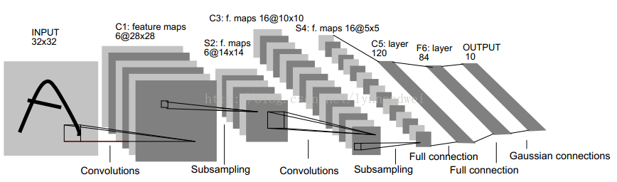
层名称	输入	卷积核/池化大小	输出	参数	连接数
C1	32×32	6，5×5，1×1	28×28×6	(5x5+1)x6=156	(5x5+1)x6x28x28=122304
S2	28×28×6	6，2×2，2×2	14×14×6	2x6=12	(2x2+1)x6x14x14=5880
C3	14×14×6	16，5×5，1×1	10×10×16	(5x5x3+1)x6 + (5x5x4 + 1) x 6 + (5x5x4 +1)x3 + (5x5x6+1)x1 = 1516	1516x10x10=151600
S4	10×10×16	16，2×2，2×2	5×5×16	2x16=32	(2x2+1)x5x5x16=2000
C5		5×5×16	120	(5x5x16+1)x120 = 48120	(5x5x16+1)x120 = 48120
F6		120	84	(120 + 1)x84=10164	(120 + 1)x84=10164
output		84	10	84x10=840	84x10=840

2.1.2 AlexNet

此处输入图片的描述

2.1.3 VGG-16

此处输入图片的描述

2.2 残差网络ResNet

由于存在梯度消失与梯度爆炸的问题，很深的神经网络是很难训练的。ResNet解决了这深层神经网络的训练问题，通过将前面层的结果通过增加的连接传递到后面更深的层次中。使得神经网络可以达到100层以上。

下图展示了残差网络的连接结构与普通网络的差别
此处输入图片的描述

上图结构的前向计算推导公式修正为:
$a^{[l+2]}=g(z^{[l+2]} + a^{[[l]})$

2.3 实现残差网络

本节我们借助于Keras实现一个残差网络-ResNet50。
此处输入图片的描述

其Identity残差块具有下面的结构。
此处输入图片的描述

其卷积残差块则具有下面的结构。
此处输入图片的描述

代码示例：

from keras.models import Model
from keras.layers import Input, Add, Dense, Activation, ZeroPadding2D, BatchNormalization, Flatten, Conv2D, AveragePooling2D, MaxPooling2D
from keras.initializers import glorot_uniform


def identity_block(X, f, filters, stage, block):
    """
    Implementation of the identity block

    Arguments:
    X -- input tensor of shape (m, n_H_prev, n_W_prev, n_C_prev)
    f -- integer, specifying the shape of the middle CONV's window for the main path
    filters -- python list of integers, defining the number of filters in the CONV layers of the main path
    stage -- integer, used to name the layers, depending on their position in the network
    block -- string/character, used to name the layers, depending on their position in the network

    Returns:
    X -- output of the identity block, tensor of shape (n_H, n_W, n_C)
    """

    # defining name basis
    conv_name_base = 'res' + str(stage) + block + '_branch'
    bn_name_base = 'bn' + str(stage) + block + '_branch'

    # Retrieve Filters
    F1, F2, F3 = filters

    # Save the input value. You'll need this later to add back to the main path.
    X_shortcut = X

    # First component of main path
    X = Conv2D(filters=F1, kernel_size=(1, 1), strides=(1, 1), padding='valid', name=conv_name_base + '2a', kernel_initializer=glorot_uniform(seed=0))(X)
    X = BatchNormalization(axis=3, name=bn_name_base + '2a')(X)
    X = Activation('relu')(X)

    # Second component of main path
    X = Conv2D(filters=F2, kernel_size=(f, f), strides=(1, 1), padding='same', name=conv_name_base + '2b', kernel_initializer=glorot_uniform(seed=0))(X)
    X = BatchNormalization(axis=3, name=bn_name_base + '2b')(X)
    X = Activation('relu')(X)

    # Third component of main path
    X = Conv2D(filters=F3, kernel_size=(1, 1), strides=(1, 1), padding='valid', name=conv_name_base + '2c', kernel_initializer=glorot_uniform(seed=0))(X)
    X = BatchNormalization(axis=3, name=bn_name_base + '2c')(X)

    # Final step: Add shortcut value to main path, and pass it through a RELU activation
    X = Add()([X, X_shortcut])
    X = Activation('relu')(X)

    return X


def convolutional_block(X, f, filters, stage, block, s=2):
    """
    Implementation of the convolutional block

    Arguments:
    X -- input tensor of shape (m, n_H_prev, n_W_prev, n_C_prev)
    f -- integer, specifying the shape of the middle CONV's window for the main path
    filters -- python list of integers, defining the number of filters in the CONV layers of the main path
    stage -- integer, used to name the layers, depending on their position in the network
    block -- string/character, used to name the layers, depending on their position in the network
    s -- Integer, specifying the stride to be used

    Returns:
    X -- output of the convolutional block, tensor of shape (n_H, n_W, n_C)
    """

    # defining name basis
    conv_name_base = 'res' + str(stage) + block + '_branch'
    bn_name_base = 'bn' + str(stage) + block + '_branch'

    # Retrieve Filters
    F1, F2, F3 = filters

    # Save the input value
    X_shortcut = X

    # First component of main path
    X = Conv2D(filters=F1, kernel_size=(1, 1), strides=(s, s), padding='valid', name=conv_name_base + '2a', kernel_initializer=glorot_uniform(seed=0))(X)
    X = BatchNormalization(axis=3, name=bn_name_base + '2a')(X)
    X = Activation('relu')(X)

    # Second component of main path
    X = Conv2D(filters=F2, kernel_size=(f, f), strides=(1, 1), padding='same', name=conv_name_base + '2b', kernel_initializer=glorot_uniform(seed=0))(X)
    X = BatchNormalization(axis=3, name=bn_name_base + '2b')(X)
    X = Activation('relu')(X)

    # Third component of main path
    X = Conv2D(filters=F3, kernel_size=(1, 1), strides=(1, 1), padding='valid', name=conv_name_base + '2c', kernel_initializer=glorot_uniform(seed=0))(X)
    X = BatchNormalization(axis=3, name=bn_name_base + '2c')(X)

    X_shortcut = Conv2D(filters=F3, kernel_size=(1, 1), strides=(s, s), padding='valid', name=conv_name_base + '1', kernel_initializer=glorot_uniform(seed=0))(X_shortcut)
    X_shortcut = BatchNormalization(axis=3, name=bn_name_base + '1')(X_shortcut)

    # Final step: Add shortcut value to main path, and pass it through a RELU activation
    X = Add()([X, X_shortcut])
    X = Activation('relu')(X)

    return X


def ResNet50(input_shape=(64, 64, 3), classes=6):
    """
    Implementation of the popular ResNet50:
    STAGE1:CONV2D -> BATCHNORM -> RELU -> MAXPOOL -> 
    STAGE2:CONVBLOCK -> IDBLOCK*2 -> 
    STAGE3:CONVBLOCK -> IDBLOCK*3 -> 
    STAGE4:CONVBLOCK -> IDBLOCK*5 ->
    STAGE5:CONVBLOCK -> IDBLOCK*2 ->
           AVGPOOL -> TOPLAYER
    """

    X_input = Input(input_shape)
    X = ZeroPadding2D((3, 3))(X_input)

    # Stage 1
    X = Conv2D(64, (7, 7), strides=(2, 2), name='conv1', kernel_initializer=glorot_uniform(seed=0))(X)
    X = BatchNormalization(axis=3, name='bn_conv1')(X)
    X = Activation('relu')(X)
    X = MaxPooling2D((3, 3), strides=(2, 2))(X)

    # Stage 2
    X = convolutional_block(X, f=3, filters=[64, 64, 256], stage=2, block='a', s=1)
    X = identity_block(X, 3, [64, 64, 256], stage=2, block='b')
    X = identity_block(X, 3, [64, 64, 256], stage=2, block='c')

    # Stage 3
    X = convolutional_block(X, f=3, filters=[128, 128, 512], stage=3, block='a', s=2)
    X = identity_block(X, 3, [128, 128, 512], stage=3, block='b')
    X = identity_block(X, 3, [128, 128, 512], stage=3, block='c')
    X = identity_block(X, 3, [128, 128, 512], stage=3, block='d')

    # Stage 4
    X = convolutional_block(X, f=3, filters=[256, 256, 1024], stage=4, block='a', s=2)
    X = identity_block(X, 3, [256, 256, 1024], stage=4, block='b')
    X = identity_block(X, 3, [256, 256, 1024], stage=4, block='c')
    X = identity_block(X, 3, [256, 256, 1024], stage=4, block='d')
    X = identity_block(X, 3, [256, 256, 1024], stage=4, block='e')
    X = identity_block(X, 3, [256, 256, 1024], stage=4, block='f')

    # Stage 5
    X = X = convolutional_block(X, f=3, filters=[512, 512, 2048], stage=5, block='a', s=2)
    X = identity_block(X, 3, [512, 512, 2048], stage=5, block='b')
    X = identity_block(X, 3, [512, 512, 2048], stage=5, block='c')

    # AVGPOOL. Use "X = AveragePooling2D(...)(X)"
    X = AveragePooling2D(pool_size=(2, 2), padding='same')(X)

    # output layer
    X = Flatten()(X)
    X = Dense(classes, activation='softmax', name='fc' + str(classes), kernel_initializer=glorot_uniform(seed=0))(X)

    # Create model
    model = Model(inputs=X_input, outputs=X, name='ResNet50')

    return model



X_train_orig, Y_train_orig, X_test_orig, Y_test_orig, classes = load_dataset()
# Normalize image vectors
X_train = X_train_orig / 255.
X_test = X_test_orig / 255.

# Convert training and test labels to one hot matrices
Y_train = convert_to_one_hot(Y_train_orig, 6).T
Y_test = convert_to_one_hot(Y_test_orig, 6).T


model = ResNet50(input_shape=(64, 64, 3), classes=6)
model.compile(optimizer='adam', loss='categorical_crossentropy', metrics=['accuracy'])
model.fit(X_train, Y_train, epochs = 2, batch_size = 32)

2.4 谷歌Inception网络

下图展示了Inception网络连接结构
此处输入图片的描述

每个Inception块的结构
此处输入图片的描述

2.5 善用开源实现

在github上已经有他人实现良好的神经网络了，如果独自实现一种神经网络有难度，不妨在github上搜索有没有人已经完成了你想做的工作。

不仅是代码，github上也有他人已经训练好的针对某些任务的模型。借助于迁移学习，可以将他人训练的模型派上用场。

zzulp

关注

0
点赞
踩
7

收藏

觉得还不错? 一键收藏
0
评论
深度学习之四：卷积神经网络基础

计算机视觉在深度学习的帮助下取得了令人惊叹的进展，其中发挥重要作用的是卷积神经网络。本节总结了卷积神经的原理与实现方法。1 卷积神经网络1.1 计算机视觉与深度学习计算机视觉要解决的问题是如何让机器理解现实世界的现象。目前主要处理的问题如图像分类，目标检测，风格变换等。对于小型图片，如MNIST的图片处理，图像大小为64*64，使用全连接神经网络还可以处理。如果图像较大，如...
复制链接

扫一扫

专栏目录