【DGL教程】第6章大图上的随机训练

最新推荐文章于 2023-12-12 21:39:02 发布

zzy979

最新推荐文章于 2023-12-12 21:39:02 发布

阅读量3k

点赞数 9

分类专栏： DGL 图神经网络文章标签： DGL 图神经网络

本文链接：https://blog.csdn.net/zzy979481894/article/details/116138705

版权

图神经网络同时被 2 个专栏收录

15 篇文章 5 订阅

订阅专栏

DGL

7 篇文章 19 订阅

订阅专栏

官方文档：https://docs.dgl.ai/guide/minibatch.html

对于有上百万甚至上亿顶点和边的图无法使用全图训练，需要使用随机minibatch训练

邻居采样方法

在每个梯度下降步骤中，如果要计算某个顶点第L层的表示，根据消息传递，需要计算其全部或部分邻居第L-1层的表示，又需要计算这些邻居的邻居第L-2层的表示……这一过程一直持续到输入层。这一迭代过程构造了一个依赖图，从输出到输入，如下图所示

DGL提供了一些邻居采样器和使用邻居采样训练GNN的方法

1.使用邻居采样的顶点分类

https://docs.dgl.ai/guide/minibatch-node.html

要使模型能够随机训练，需要：

定义一个邻居采样器
将模型适配minibatch训练
修改训练循环

1.1 定义邻居采样器和数据加载器

dgl.dataloading.neighbor模块提供了几个邻居采样器类，给定希望计算的顶点，能够生成每一层需要的计算依赖图
最简单的邻居采样器是MultiLayerFullNeighborSampler，直接选择顶点在每一层的所有邻居
数据加载器使用NodeDataLoader，用于以minibatch的形式迭代训练顶点集合

示例：
顶点分类原图

>>> import dgl
>>> import torch
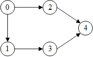
>>> g = dgl.graph((torch.tensor([0, 0, 1, 2, 3]), torch.tensor([1, 2, 3, 4, 4])))
>>> g
Graph(num_nodes=5, num_edges=5,
      ndata_schemes={}
      edata_schemes={})
>>> train_nids = torch.tensor([3, 4])
>>> from dgl.dataloading import MultiLayerFullNeighborSampler, NodeDataLoader
>>> sampler = MultiLayerFullNeighborSampler(2)
>>> dataloader = NodeDataLoader(g, train_nids, sampler, batch_size=1)
>>> it = iter(dataloader)

第1次迭代（第1个batch）：目标顶点是3，由于网络层数（邻居采样器的参数）是2，因此需要计算两层的依赖关系，从后往前计算：第2层只需要3的邻居1，第1层还需要1的邻居0
每次迭代器生成三项：input_nodes, output_nodes, blocks

output_nodes是batch中的目标顶点，即需要计算表示的顶点（最后一层的输出顶点）
input_nodes是计算这些顶点的表示所需要的输入顶点（第1层的输入顶点）
blocks是每一层GNN的输入图，第i个block由第i层的输入顶点和第i层的输出顶点（第i+1层的输入顶点）组成
input_nodes对应blocks[0].srcnodes()，output_nodes对应blocks[-1].dstnodes()，但input_nodes始终将output_nodes放在最前面，即input_nodes[:len(output_nodes)] == output_nodes
dataloader生成的block对顶点进行了重新编号，原id保存在名为dgl.NID的顶点属性中

>>> input_nodes, output_nodes, blocks = next(it)
>>> input_nodes
tensor([3, 1, 0])
>>> output_nodes
tensor([3])
>>> blocks
[Block(num_src_nodes=3, num_dst_nodes=2, num_edges=2), Block(num_src_nodes=2, num_dst_nodes=1, num_edges=1)]
>>> blocks[0].edges()
(tensor([1, 2]), tensor([0, 1]))
>>> blocks[0].ndata[dgl.NID]
{'_N': tensor([3, 1, 0])}
>>> blocks[1].edges()
(tensor([1]), tensor([0]))
>>> blocks[1].ndata[dgl.NID]
{'_N': tensor([3, 1])}

第2次迭代的目标顶点是4，依赖关系的计算方式同上
顶点分类batch 2

>>> input_nodes, output_nodes, blocks = next(it)
>>> input_nodes
tensor([4, 2, 3, 0, 1])
>>> output_nodes
tensor([4])
>>> blocks[0].edges()
(tensor([1, 2, 3, 4]), tensor([0, 0, 1, 2]))
>>> blocks[0].ndata[dgl.NID]
{'_N': tensor([4, 2, 3, 0, 1])}
>>> blocks[1].edges()
(tensor([1, 2]), tensor([0, 0]))
>>> blocks[1].ndata[dgl.NID]
{'_N': tensor([4, 2, 3])}

1.2 将模型适配minibatch训练

假设有以下全图训练的两层GCN模型：

class GCN(nn.Module):

    def __init__(self, in_feats, hidden_size, num_classes):
        super().__init__()
        self.conv1 = GraphConv(in_feats, hidden_size)
        self.conv2 = GraphConv(hidden_size, num_classes)

    def forward(self, g, inputs):
        h = self.conv1(g, inputs)
        h = F.relu(h)
        h = self.conv2(g, h)
        return h

要使模型适配minibatch训练，只需要将forward函数的参数g改为blocks，并将每层的输入分别改为blocks[0], blocks[1]...即可，如下：

class GCN(nn.Module):

    def __init__(self, in_feats, hidden_size, num_classes):
        super().__init__()
        self.conv1 = GraphConv(in_feats, hidden_size)
        self.conv2 = GraphConv(hidden_size, num_classes)

    def forward(self, blocks, inputs):
        h = self.conv1(blocks[0], inputs)
        h = F.relu(h)
        h = self.conv2(blocks[1], h)
        return h

Q: GraphConv的输入图顶点个数与输入特征大小不同？
A: DGL内置图卷积模块都支持全图训练和minibatch训练两种模式，如果输入图是block则只取终点的特征
以下代码来自SAGEConv.forward()：

if graph.is_block:
    feat_dst = feat_src[:graph.number_of_dst_nodes()]

为保证这样做是正确的，采样器会将终点id放在最前面

1.3 训练循环

使用blocks[0].srcdata获取输入特征
将blocks和顶点输入特征输入多层GNN，获取输出
使用blocks[-1].dstdata获取输出顶点表示
计算损失和反向传播

Q: forward参数改为blocks后如何进行验证集和测试集的评价？
A: 为验证集和测试集都分别创建一个DataLoader

完整代码：
https://github.com/dmlc/dgl/blob/master/examples/pytorch/graphsage/train_sampling.py
https://github.com/ZZy979/pytorch-tutorial/blob/master/gnn/dgl/node_clf_mb.py

1.4 异构图

异构图的邻居采样方法与同构图类似，也是将模型的forward函数的参数改为blocks
另外，NodeCollator的训练顶点id参数不是一个张量而是一个顶点类型到张量的字典，迭代生成的input_nodes和output_nodes也都是字典

完整代码：
https://github.com/dmlc/dgl/blob/master/examples/pytorch/rgcn-hetero/entity_classify_mb.py
https://github.com/ZZy979/pytorch-tutorial/blob/master/gnn/dgl/node_clf_hetero_mb.py

2.使用邻居采样的边分类

https://docs.dgl.ai/en/latest/guide/minibatch-edge.html

2.1 定义邻居采样器和数据加载器

邻居采样器仍然可以使用MultiLayerFullNeighborSampler
而数据加载器要使用EdgeDataLoader，用于以minibatch的形式迭代训练边集合，并生成边子图和MFG

示例：
边分类原图

>>> import dgl
>>> import torch
>>> g = dgl.graph((torch.tensor([0, 1, 1, 2, 3]), torch.tensor([1, 2, 3, 0, 2])))
>>> g
Graph(num_nodes=4, num_edges=5,
      ndata_schemes={}
      edata_schemes={})
>>> train_eids = torch.tensor([1, 2])
>>> from dgl.dataloading import MultiLayerFullNeighborSampler, EdgeDataLoader
>>> sampler = MultiLayerFullNeighborSampler(2)
>>> dataloader = EdgeDataLoader(g, train_eids, sampler, batch_size=1)
>>> it = iter(dataloader)

每次迭代生成三项：input_nodes, edge_subgraph, blocks

input_nodes和blocks分别是第1层的输入顶点和每一层的MFG，与NodeDataLoader相同
edge_subgraph是仅包含当前batch中边及其端点的子图，原始顶点id和边id分别被保存在名为dgl.NID的顶点特征和名为dgl.EID的边特征中

第1个batch的边id是1，为了计算边1的特征，需要其两端点1和2的特征（相乘、内积等），因此顶点1和2是目标顶点，对应的边子图和两层MFG如下：
边分类batch 1
（注：边子图中边上的数字表示原图中的边id，block中的顶点id是未重新编号之前的）

>>> input_nodes, edge_subgraph, blocks = next(it)
>>> input_nodes
tensor([1, 2, 0, 3])
>>> edge_subgraph
Graph(num_nodes=2, num_edges=1,
      ndata_schemes={'_ID': Scheme(shape=(), dtype=torch.int64)}
      edata_schemes={'_ID': Scheme(shape=(), dtype=torch.int64)})
>>> edge_subgraph.edges()
(tensor([0]), tensor([1]))
>>> edge_subgraph.ndata[dgl.NID]
tensor([1, 2])
>>> edge_subgraph.edata[dgl.EID]
tensor([1])
>>> blocks
[Block(num_src_nodes=4, num_dst_nodes=4, num_edges=5), Block(num_src_nodes=4, num_dst_nodes=2, num_edges=3)]
>>> blocks[0].edges()
(tensor([2, 0, 3, 1, 0]), tensor([0, 1, 1, 2, 3]))
>>> blocks[0].ndata[dgl.NID]
{'_N': tensor([1, 2, 0, 3])}
>>> blocks[1].edges()
(tensor([2, 0, 3]), tensor([0, 1, 1]))
>>> blocks[1].ndata[dgl.NID]
{'_N': tensor([1, 2, 0, 3])}

第2个batch的边id是2，因此其端点1和3是目标顶点：
边分类batch 2

>>> input_nodes, edge_subgraph, blocks = next(it)
>>> edge_subgraph
Graph(num_nodes=2, num_edges=1,
      ndata_schemes={'_ID': Scheme(shape=(), dtype=torch.int64)}
      edata_schemes={'_ID': Scheme(shape=(), dtype=torch.int64)})
>>> edge_subgraph.edges()
(tensor([0]), tensor([1]))
>>> edge_subgraph.ndata[dgl.NID]
tensor([1, 3])
>>> edge_subgraph.edata[dgl.EID]
tensor([2])
>>> blocks
[Block(num_src_nodes=4, num_dst_nodes=3, num_edges=3), Block(num_src_nodes=3, num_dst_nodes=2, num_edges=2)]
>>> blocks[0].edges()
(tensor([2, 0, 3]), tensor([0, 1, 2]))
>>> blocks[0].ndata[dgl.NID]
{'_N': tensor([1, 3, 0, 2])}
>>> blocks[1].edges()
(tensor([2, 0]), tensor([0, 1]))
>>> blocks[1].ndata[dgl.NID]
{'_N': tensor([1, 3, 0])}

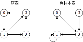
在邻居采样时从原图中移除batch中的边

在训练边分类模型时，有时需要将训练数据中出现的边从MFG中移除，否则模型会“知道”两个顶点之间存在边
为此，在实例化EdgeDataLoader时指定exclude参数，则生成的blocks中将不存在batch中的边

仍然以上面的图为例
边分类batch 1
和之前的唯一区别是block中删除了顶点1和2之间的边

>>> dataloader = EdgeDataLoader(g, train_eids, sampler, exclude='self', batch_size=1)
>>> it = iter(dataloader)
>>> input_nodes, edge_subgraph, blocks = next(it)
>>> blocks[0].edges()
(tensor([2, 3, 1, 0]), tensor([0, 1, 2, 3]))
>>> blocks[0].ndata[dgl.NID]
{'_N': tensor([1, 2, 0, 3])}
>>> blocks[1].edges()
(tensor([2, 3]), tensor([0, 1]))
>>> blocks[1].ndata[dgl.NID]
{'_N': tensor([1, 2, 0, 3])}

边分类batch 2

>>> input_nodes, edge_subgraph, blocks = next(it)
>>> blocks[0].edges()
(tensor([2, 3]), tensor([0, 2]))
>>> blocks[0].ndata[dgl.NID]
{'_N': tensor([1, 3, 0, 2])}
>>> blocks[1].edges()
(tensor([2]), tensor([0]))
>>> blocks[1].ndata[dgl.NID]
{'_N': tensor([1, 3, 0])}

2.2 将模型适配mini-batch训练

边分类模型通常由两部分组成：

一部分计算顶点的表示（GNN模型）
另一部分由顶点表示计算边上的得分（如内积）

第一部分仍然使用1.2节中的两层GCN模型，第二部分的输入通常是第一部分输出的顶点表示以及minibatch中的边构造的边子图，可直接使用“训练GNN”2.1节中的MLPPredictor
整体模型将GCN和MLPPredictor连接在一起即可

class Model(nn.Module):

    def __init__(self, in_features, hidden_features, out_features, num_classes):
        super().__init__()
        self.gcn = GCN(in_features, hidden_features, out_features)
        self.pred = MLPPredictor(out_features, num_classes)

    def forward(self, edge_subgraph, blocks, h):
        h = self.gcn(blocks, h)
        return self.pred(edge_subgraph, h)

2.3 训练循环

迭代dataloader，每个batch生成input_nodes, edge_subgraph, blocks三项
使用blocks[0].srcdata['feat']获取顶点输入特征
将edge_subgraph, blocks和顶点输入特征输入GNN模型，获取输出的边表示
使用edge_subgraph.edata['label']获取边标签
计算损失和反向传播

完整代码：https://github.com/ZZy979/pytorch-tutorial/blob/master/gnn/dgl/edge_clf_mb.py

2.4 异构图

异构图上使用邻居采样的边分类与同构图非常类似，只是EdgeDataLoader的训练边id参数是一个边类型到张量的映射，迭代生成的input_nodes也是字典，而edge_subgraph和blocks都是异构图

计算顶点表示的模型可使用“训练GNN”1.2节中RGCN的minibatch版本，得分预测可直接使用“训练GNN”2.2节中的HeteroDotProductPredictor

完整代码：https://github.com/ZZy979/pytorch-tutorial/blob/master/gnn/dgl/edge_clf_hetero_mb.py

3.使用邻居采样的连接预测

https://docs.dgl.ai/en/latest/guide/minibatch-link.html

3.1 定义邻居采样器和带有负采样的数据加载器

邻居采样器仍然可以使用MultiLayerFullNeighborSampler
DGL中的EdgeDataLoader支持生成用于连接预测的负样本，为此，需要指定negative_sampler参数
dgl.dataloading.negative_sampler.Uniform是DGL内置的负采样器，对于每条边(u, v)，采样k个负样本边(u, v1’), …, (u, vk’)，即原图中不存在的边
其（简化的）实现如下：

class Uniform:

    def __init__(self, k):
        self.k = k

    def __call__(self, g, eids):
        src, _ = g.find_edges(eids)
        src = src.repeat_interleave(self.k)
        dst = torch.randint(0, graph.num_nodes(), (len(src),))
        return src, dst

负采样器示例：

>>> g = dgl.graph((torch.tensor([0, 1, 1, 2, 3]), torch.tensor([1, 2, 3, 0, 2])))
>>> neg_sampler = Uniform(1)
>>> neg_sampler(g, torch.arange(g.num_edges()))
(tensor([0, 1, 1, 2, 3]), tensor([3, 0, 1, 3, 1]))

使用负采样的EdgeDataLoader示例：
图和训练边id与2.1节完全相同，只是增加了负采样
连接预测原图

>>> import dgl
>>> import torch
>>> g = dgl.graph((torch.tensor([0, 1, 1, 2, 3]), torch.tensor([1, 2, 3, 0, 2])))
>>> g
Graph(num_nodes=4, num_edges=5,
      ndata_schemes={}
      edata_schemes={})
>>> train_eids = torch.tensor([1, 2])
>>> from dgl.dataloading import MultiLayerFullNeighborSampler, EdgeDataLoader
>>> from dgl.dataloading.negative_sampler import Uniform
>>> sampler = MultiLayerFullNeighborSampler(2)
>>> dataloader = EdgeDataLoader(g, train_eids, sampler, negative_sampler=Uniform(2), batch_size=1)
>>> it = iter(dataloader)

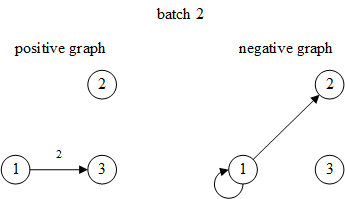
每次迭代生成四项：input_nodes, positive_graph, negative_graph, blocks

input_nodes和blocks与边分类相同
positive_graph就是edge_subgraph，即仅包含当前batch中边及其端点的子图
negative_graph是负样本边组成的负样本图

第1个batch（input_nodes和blocks与2.1节相同，这里不再展示）：
连接预测batch 1

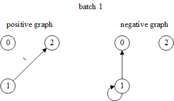
>>> input_nodes, positive_graph, negative_graph, blocks = next(it)
>>> positive_graph.edges()
(tensor([0]), tensor([1]))
>>> positive_graph.ndata[dgl.NID]
tensor([1, 2, 0])
>>> positive_graph.edata[dgl.EID]
tensor([1])
>>> negative_graph.edges()
(tensor([0, 0]), tensor([2, 0]))
>>> negative_graph.ndata[dgl.NID]
tensor([1, 2, 0])

第2个batch：
连接预测batch 2

>>> input_nodes, positive_graph, negative_graph, blocks = next(it)
>>> positive_graph.edges()
(tensor([0]), tensor([1]))
>>> positive_graph.ndata[dgl.NID]
tensor([1, 3, 2])
>>> positive_graph.edata[dgl.EID]
tensor([2])
>>> negative_graph.edges()
(tensor([0, 0]), tensor([0, 2]))
>>> negative_graph.ndata[dgl.NID]
tensor([1, 3, 2])

3.2 将模型适配mini-batch训练

连接预测的训练目标是比较正样本边的得分和负样本边的得分，可以复用边分类模型计算的顶点表示和边得分，与边分类模型唯一的区别是得分预测模块需要分别计算正样本图和负样本图中边的得分

class Model(nn.Module):

    def __init__(self, in_features, hidden_features, out_features):
        super().__init__()
        self.gcn = GCN(in_features, hidden_features, out_features)
        self.pred = DotProductPredictor()

    def forward(self, pos_g, neg_g, blocks, x):
        h = self.gcn(blocks, x)
        return self.pred(pos_g, h), self.pred(neg_g, h)

3.3 训练循环

迭代dataloader，每个batch生成input_nodes, pos_g, neg_g, blocks四项
使用blocks[0].srcdata['feat']获取顶点输入特征
将pos_g, neg_g, blocks和顶点输入特征输入GNN模型，获取输出的边预测得分
计算损失和反向传播

完整代码：https://github.com/ZZy979/pytorch-tutorial/blob/master/gnn/dgl/link_pred_mb.py

3.4 异构图

异构图上使用邻居采样的连接预测与同构图非常类似，只是EdgeDataLoader的训练边id参数是一个边类型到张量的映射，迭代生成的input_nodes也是字典，而positive_graph, negative_graph和blocks都是异构图
如果输入负采样器的图是异构图，则采样出的负样本图也是异构图

完整代码：https://github.com/ZZy979/pytorch-tutorial/blob/master/gnn/dgl/link_pred_hetero_mb.py

4.自定义邻居采样器

https://docs.dgl.ai/en/latest/guide/minibatch-custom-sampler.html

4.1 邻居采样的基本概念

要使用mini-batch方法进行多层消息传递，需要将顶点集合划分为多个batch，每次只计算一个batch的顶点的输出，这一个batch的顶点称为目标顶点或种子顶点(seed node)

例如，在下图中要计算目标顶点8的输出
原始图
根据消息传递公式，需要聚集来自顶点8的邻居N(8)={4, 5, 7, 11}的消息，如下图所示
一阶邻居消息传递
该图包含了原图中的所有顶点，但只有到目标顶点的消息传递所需要的边，这种图称为frontier
可以生成frontier图的函数有dgl.in_subgraph()和dgl.sampling.sample_neighbors()，区别是前者保留所有邻居（入边），后者可以对邻居采样

>>> u = [0, 0, 0, 1, 2, 2, 2, 3, 3, 4, 4, 5, 5, 6, 7, 7, 8, 9, 10]
>>> v = [1, 2, 3, 3, 3, 4, 5, 5, 6, 5, 8, 6, 8, 9, 8, 11, 11, 10, 11]
>>> g = dgl.to_bidirected(dgl.graph((u, v)))
>>> g
Graph(num_nodes=12, num_edges=38,
      ndata_schemes={}
      edata_schemes={})
>>> frontier = dgl.in_subgraph(g, [8])
>>> frontier
Graph(num_nodes=12, num_edges=4,
      ndata_schemes={}
      edata_schemes={'_ID': Scheme(shape=(), dtype=torch.int64)})
>>> frontier.edges()
(tensor([ 4,  5,  7, 11]), tensor([8, 8, 8, 8]))
>>> frontier2 = dgl.sampling.sample_neighbors(g, [8], fanout=2)
>>> frontier2
Graph(num_nodes=12, num_edges=2,
      ndata_schemes={}
      edata_schemes={'_ID': Scheme(shape=(), dtype=torch.int64)})
>>> frontier2.edges()
(tensor([11,  5]), tensor([8, 8]))

所有的子图构造和采样操作见 Subgraph Extraction Ops 和 dgl.sampling

要计算目标顶点的输出特征，不能直接在frontier图上进行消息传递，因为frontier图包含原图的所有顶点（可能有上百万），实际上只需要目标顶点及其邻居作为输入顶点(input/source nodes)、目标顶点作为输出顶点(output/destination nodes)的这样一个二分结构的图即可，这样的图称为消息流图(message flow graph, MFG)或block
在上面的例子中，为了计算目标顶点8的输出特征，只需要下图所示的MFG即可
MFG示例

DGL提供了dgl.to_block()函数来将frontier转换为MFG (block)

>>> block = dgl.to_block(frontier, [8])
>>> block
Block(num_src_nodes=5, num_dst_nodes=1, num_edges=4)
>>> block.srcdata[dgl.NID]
tensor([ 8,  4,  5,  7, 11])
>>> block.dstdata[dgl.NID]
tensor([8])

注意：

目的顶点也会出现在源顶点中（开头部分）

>>> torch.equal(block.dstdata[dgl.NID], block.srcdata[dgl.NID][:block.num_dst_nodes()])
True

block将源顶点和目的顶点视为不同的类型（但是类型名称一样），因此源顶点8和目的顶点8不是同一个顶点
```
>>> block.ntypes, block.srctypes, block.dsttypes
(['_N', '_N'], ['_N'], ['_N'])
```
顶点在原图中的id会被保存在名为dgl.NID的顶点特征中
由于block是一种二分图，访问顶点和顶点特征要区分源顶点和目的顶点

	普通图	二分图
顶点	g.nodes()	g.srcnodes(), g.dstnodes()
顶点数	g.num_nodes()	g.num_src_nodes(), g.num_dst_nodes()
顶点特征	g.ndata	g.srcdata, g.dstdata
异构顶点特征	g.nodes[ntype].data	g.srcnodes[ntype].data, g.dstnodes[ntype].data

dgl.to_block()也可用于异构图，此时第二个参数应当是顶点类型到顶点id列表的映射

4.2 邻居采样器

1.1节展示了邻居采样器的用法，这里解释其实现原理

邻居采样器的基类是BlockSampler，其功能是根据指定的目标顶点（最后一层的输出顶点）生成每一层的MFG，（简化的）定义如下：

class BlockSampler(object):

    def __init__(self, num_layers):
        self.num_layers = num_layers

    def sample_frontier(self, block_id, g, seed_nodes):
        raise NotImplementedError

    def sample_blocks(self, g, seed_nodes, exclude_eids=None):
        blocks = []
        for block_id in reversed(range(self.num_layers)):
            frontier = self.sample_frontier(block_id, g, seed_nodes)
            block = transform.to_block(frontier, seed_nodes)
            seed_nodes = {ntype: block.srcnodes[ntype].data[NID] for ntype in block.srctypes}
            blocks.insert(0, block)
        return blocks

该类有两个方法：

sample_frontier()：给定原图和目标顶点生成frontier，这是抽象方法，与具体的邻居采样策略有关
sample_blocks()：给定原图和目标顶点，生成每一层的MFG，该类已经提供了默认实现，就是从最后一层开始反向迭代，依次生成每一层的frontier并转换为block

例如，对于下面的图，目标顶点为8，层数为2，则第2层MFG是绿色顶点到红色顶点的二分图，第1层MFG是黄色顶点到绿色顶点的二分图
两层消息传递示例

这里的“层数”对应GNN模型的层数，生成的block列表分别作为每一层GNN的输入图

4.1节中提到dgl.in_subgraph()和dgl.sampling.sample_neighbors()是生成frontier的两种方式，分别是保留所有邻居和采样邻居，这就是MultiLayerFullNeighborSampler和MultiLayerNeighborSampler的实现方式（与实际实现稍有差别）：

class MultiLayerFullNeighborSampler(dgl.dataloading.BlockSampler):

    def __init__(self, n_layers):
        super().__init__(n_layers)

    def sample_frontier(self, block_id, g, seed_nodes):
        return dgl.in_subgraph(g, seed_nodes)


class MultiLayerNeighborSampler(dgl.dataloading.BlockSampler):

    def __init__(self, fanouts):
        super().__init__(len(fanouts))
        self.fanouts = fanouts

    def sample_frontier(self, block_id, g, seed_nodes):
        fanout = self.fanouts[block_id]
        return dgl.sampling.sample_neighbors(g, seed_nodes, fanout)

要实现自定义的邻居采样器，只要继承BlockSampler类，并实现sample_frontier()方法即可，在该方法中实现自定义的邻居采样策略

4.3 NodeCollator和NodeDataLoader

collator是PyTorch的DataLoader中的概念（collate_fn参数），作用是将DataLoader的迭代器生成的每个batch的数据处理成可以作为模型输入的形式

一般情况下，训练样本是tensor(N, d)，DataLoader生成的每个batch的数据是tensor(B, d)，已经可以直接作为模型输入，不需要其他处理，因此不需要设置collate_fn参数
但是对于GNN模型来说，每个batch的数据是目标顶点id，而输入到模型的“训练样本”是这些目标顶点对应的多层MFG及其顶点特征，因此需要使用邻居采样器生成给定目标顶点的多层MFG，这就是NodeCollator的作用，其（简化的）定义如下：

class NodeCollator(Collator):

    def __init__(self, g, nids, block_sampler):
        self.g = g
        self.block_sampler = block_sampler
        self._dataset = nids

    @property
    def dataset(self):
        return self._dataset

    def collate(self, items):
        blocks = self.block_sampler.sample_blocks(self.g, items)
        output_nodes = blocks[-1].dstdata[NID]
        input_nodes = blocks[0].srcdata[NID]
        return input_nodes, output_nodes, blocks

核心方法是collate()，逻辑很简单，就是使用邻居采样器生成给定目标顶点(items)对应的多层MFG (blocks)（层数由邻居采样器指定），并附加了第一层的输入顶点和最后一层的输出顶点作为返回值

使用时将collate()方法作为DataLoader的collate_fn参数即可：

sampler = MultiLayerFullNeighborSampler(2)
collator = NodeCollator(g, train_nids, sampler)
dataloader = DataLoader(collator.dataset, batch_size=32, collate_fn=collator.collate)
for input_nodes, blocks in dataloader:
    logits = model(blocks, blocks[0].srcdata['feat'])
    # ...

DGL提供了NodeDataLoader类自动实现了NodeCollator和DataLoader的组合，其（简化的）定义如下：

class NodeDataLoader:

    def __init__(self, g, nids, block_sampler):
        self.collator = NodeCollator(g, nids, block_sampler)
        self.dataloader = DataLoader(self.collator.dataset, collate_fn=self.collator.collate)

    def __iter__(self):
        return iter(self.dataloader)

    def __len__(self):
        return len(self.dataloader)

因此不需要手动创建NodeCollator：

dataloader = NodeDataLoader(g, train_nids, sampler, batch_size=32)

4.4 异构图

生成异构图的frontier与同构图基本没有区别，只是目标顶点id应当是顶点类型到顶点id的映射，NodeCollator返回的input_nodes和output_nodes也都是字典

5.实现用于mini-batch训练的自定义GNN模块

https://docs.dgl.ai/en/latest/guide/minibatch-nn.html
MFG上的计算代码与全图类似，除了顶点分为输入顶点和输出顶点

5.1 同构图

以下是一个自定义图卷积模块的实例（输出特征=输入特征与邻居平均的拼接+线性变换）：

class CustomGraphConv(nn.Module):
    def __init__(self, in_feats, out_feats):
        super().__init__()
        self.W = nn.Linear(in_feats * 2, out_feats)

    def forward(self, g, h):
        with g.local_scope():
            g.ndata['h'] = h
            g.update_all(fn.copy_u('h', 'm'), fn.mean('m', 'h_neigh'))
            return self.W(torch.cat([g.ndata['h'], g.ndata['h_neigh']], 1))

将其修改为用于MFG的版本：

class CustomGraphConv(nn.Module):
    def __init__(self, in_feats, out_feats):
        super().__init__()
        self.W = nn.Linear(in_feats * 2, out_feats)

    def forward(self, block, h):
        with block.local_scope():
            block.srcdata['h'] = h
            block.dstdata['h'] = h[:block.num_dst_nodes()]
            block.update_all(fn.copy_u('h', 'm'), fn.mean('m', 'h_neigh'))
            return self.W(torch.cat([block.dstdata['h'], block.dstdata['h_neigh']], 1))

一般地，要将GNN模块改为用于MFG的版本，需要执行以下操作：

从输入顶点特征的前几行获取输出顶点的特征：h_dst = h[:block.num_dst_nodes()]
如果原图只有一种顶点类型或是二分图，则将g.ndata对于输入顶点替换为block.srcdata，对于输出顶点替换为block.dstdata
如果原图有多种顶点类型，则将g.ndata对于输入顶点替换为block.srcnodes[stype].data，对于输出顶点替换为block.dstnodes[dtype].data
将g.num_nodes()对于输入和输出顶点分别替换为block.num_src_nodes()和block.num_dst_nodes()

5.2 异构图

考虑以下用于全图的模块：

class CustomHeteroGraphConv(nn.Module):
    def __init__(self, g, in_feats, out_feats):
        super().__init__()
        self.Ws = nn.ModuleDict()
        self.Vs = nn.ModuleDice()
        for utype, etype, vtype in g.canonical_etypes:
            self.Ws[etype] = nn.Linear(in_feats[utype], out_feats[vtype])
        for ntype in g.ntypes:
            self.Vs[ntype] = nn.Linear(in_feats[ntype], out_feats[ntype])

    def forward(self, g, h):
        with g.local_scope():
            for ntype in g.ntypes:
                g.nodes[ntype].data['h_src'] = h[ntype]
                g.nodes[ntype].data['h_dst'] = self.Vs[ntype](h[ntype])
            for utype, etype, vtype in g.canonical_etypes:
                g.update_all(fn.copy_u('h_src', 'm'), fn.mean('m', 'h_neigh'), etype=etype)
                g.nodes[vtype].data['h_dst'] += self.Ws[etype](g.nodes[vtype].data['h_neigh'])
            return {ntype: g.nodes[ntype].data['h_dst'] for ntype in g.ntypes}

修改原则是将g.nodes替换为g.srcnodes或g.dstnodes

class CustomHeteroGraphConv(nn.Module):
    def __init__(self, g, in_feats, out_feats):
        super().__init__()
        self.Ws = nn.ModuleDict()
        self.Vs = nn.ModuleDice()
        for utype, etype, vtype in g.canonical_etypes:
            self.Ws[etype] = nn.Linear(in_feats[utype], out_feats[vtype])
        for ntype in g.ntypes:
            self.Vs[ntype] = nn.Linear(in_feats[ntype], out_feats[ntype])

    def forward(self, block, h):
        with block.local_scope():
            for ntype in block.ntypes:
                block.srcnodes[ntype].data['h_src'] = h[ntype]
                block.dstnodes[ntype].data['h_dst'] = self.Vs[ntype](h[ntype][:block.num_dst_nodes(ntype=ntype)])
            for utype, etype, vtype in block.canonical_etypes:
                block.update_all(fn.copy_u('h_src', 'm'), fn.mean('m', 'h_neigh'), etype=etype)
                block.dstnodes[vtype].data['h_dst'] += self.Ws[etype](block.dstnodes[vtype].data['h_neigh'])
            return {ntype: block.dstnodes[ntype].data['h_dst'] for ntype in block.ntypes}

5.3 编写能够用于同构图、二分图和MFG的模块

DGL内置的卷积模块都支持同构图、二分图和有一种边类型的MFG
本质上，DGL内置卷积模块的输入图和属性必须满足以下情况之一：

如果输入特征是一对张量(feat_src, feat_dst)，则输入图必须是二分图
如果输入特征是单个向量、输入图是MFG，DGL会自动获取输出顶点特征h_dst = h[:g.num_dst_nodes()]
输入特征是单个张量、输入图不是MFG，则输入图必须是同构图

简化的SAGEConv如下：

class SAGEConv(nn.Module):
    def __init__(self, in_feats, out_feats):
        super().__init__()
        self.W = nn.Linear(in_feats * 2, out_feats)

    def forward(self, g, h):
        if isinstance(h, tuple):
            h_src, h_dst = h
        elif g.is_block:
            h_src = h
            h_dst = h[:g.num_dst_nodes()]
        else:
            h_src = h_dst = h

        g.srcdata['h'] = h_src
        g.dstdata['h'] = h_dst
        g.update_all(fn.copy_u('h', 'm'), fn.sum('m', 'h_neigh'))
        return F.relu(self.W(torch.cat([g.dstdata['h'], g.dstdata['h_neigh']], 1)))

6.大图上的精确离线推断

https://docs.dgl.ai/en/latest/guide/minibatch-inference.html
子图采样和邻居采样都是为了减少使用GPU训练GNN的内存和时间开销，而进行推断(inference)时最好真正聚集所有邻居，从而避免采样带来的随机性
然而由于GPU的内存限制，全图前向传播通常是不可行的，因此需要在有限的GPU内存下通过minibatch和邻居采样进行全图前向传播

推断算法与训练算法不同，训练算法的外层循环按顶点的minibatch迭代，内层循环（在GNN模型的forward函数中）按层迭代（消息传递/邻居采样）；而推断算法相反，外层循环按层迭代，内层循环按顶点的minibatch迭代

离线推断的实现

考虑一个两层GCN，实现离线推断仍然需要MultiLayerFullNeighborSampler（不进行邻居采样），但一次只为一层采样
注意离线推断实现为GNN模型的一个方法，因为每层上的计算依赖于消息传递

class StochasticTwoLayerGCN(nn.Module):
    def __init__(self, in_features, hidden_features, out_features):
        super().__init__()
        self.hidden_features = hidden_features
        self.out_features = out_features
        self.conv1 = dgl.nn.GraphConv(in_features, hidden_features)
        self.conv2 = dgl.nn.GraphConv(hidden_features, out_features)
        self.n_layers = 2

    def forward(self, blocks, x):
        x = F.relu(self.conv1(blocks[0], x))
        x = F.relu(self.conv2(blocks[1], x))
        return x

    def inference(self, g, x, batch_size, device):
        """
        Offline inference with this module
        """
        # Compute representations layer by layer
        for l, layer in enumerate([self.conv1, self.conv2]):
            y = torch.zeros(g.num_nodes(),
                            self.hidden_features
                            if l != self.n_layers - 1
                            else self.out_features)
            sampler = dgl.dataloading.MultiLayerFullNeighborSampler(1)
            dataloader = dgl.dataloading.NodeDataLoader(
                g, torch.arange(g.num_nodes()), sampler,
                batch_size=batch_size)

            # Within a layer, iterate over nodes in batches
            for input_nodes, output_nodes, blocks in dataloader:
                block = blocks[0]
                # Copy the features of necessary input nodes to GPU
                h = x[input_nodes].to(device)
                # Compute output.  Note that this computation is the same
                # but only for a single layer.
                h = F.relu(layer(block, h))
                # Copy to output back to CPU.
                y[output_nodes] = h.cpu()
            x = y
        return y

zzy979

关注

9
点赞
踩
24

收藏

觉得还不错? 一键收藏
1
评论
【DGL教程】第6章大图上的随机训练

官方文档：https://docs.dgl.ai/guide/minibatch.html对于有上百万甚至上亿顶点和边的图无法使用全图训练，需要使用随机minibatch训练邻居采样方法在每个梯度下降步骤中，如果要计算某个顶点第L层的表示，根据消息传递，需要计算其全部或部分邻居第L-1层的表示，又需要计算这些邻居的邻居第L-2层的表示……这一过程一直持续到输入层。这一迭代过程构造了一个依赖图，从输出到输入，如下图所示DGL提供了一些邻居采样器和使用邻居采样训练GNN的方法1.使用邻居采样的顶点分
复制链接

扫一扫