逻辑回归（logistic regression)

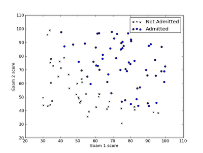
逻辑回归和线性回归的差异就是预测模型h的输出，前者输出0和1两个离散值，而线性回归输出连续值。在为分类预测建立模型时候，显然线性回归学习就不是很适合，要用逻辑回归学习算法。例如将下面数据分类：

先看看逻辑回归的预测模型吧：

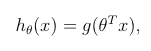
x是预测对象的features。g(x)函数是大名鼎鼎的S型函数（sigmoid function):

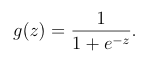
看图直观感受一下这个函数：

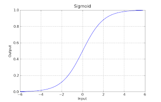
从图就可以看书，g(z)的值大部分都在0和1附近，这就是为什么我们的预测模型h(x)可以很适合输出离散值去预测分类问题了。

好了，模型有了，下面的主要任务就是确定模型中theta的值，这就是学习算法的主要任务。

同线性回归一样，需要设计一个代价函数（cost function），然后需要计算每个theta对应的梯度（gradient）

代价函数这样设计：

然后求theta变量的梯度，如果你的高数学的比较好，你可以自己推导求出梯度gradient，对照是不是下面这个结果：

现在问题来了，为什么要求梯度？

在线性回归中我们了解到，求出梯度后利用梯度做“梯度下降”算法，更新theta值，最终优化代价函数J(theta)，使J(theta)的值最小。

在这儿求梯度也是同样的道理。

Python中的scipy模块中的fmin_bfgs函数可以优化J(theta)是其最小，我们只要把J(theta)函数和梯度gradient最为参数传给fmin_bfgs这个函数就行了。

优化完毕后，得到theta值。

有了theta值，我们就可以预测新的数据X了，就是theta和X代入模型，小学生都会。

theta*X=0就是决策边界（decision boundary），画出来看一看更直观：

具体实现细节看下面代码：（代码中用到的数据“ex2data1.txt"可以在这里下载）

__author__ = 'jianyong'

# machine learning -- logistic regression by python
import numpy as np
import pylab as pl

# load and visit data
data=np.loadtxt('ex2data1.txt',delimiter=',')

X=data[:,0:2]
y=data[:,2]

pos=np.where(y==1)
neg=np.where(y==0)

pl.scatter(X[pos,0],X[pos,1],marker='o',c='b')
pl.scatter(X[neg,0],X[neg,1],marker='x',c='r')

pl.xlabel('exam1 score')
pl.ylabel('exam2 score')
pl.legend(['admitted','not admitted'])
pl.show()

# sigmoid function cost function and gradient function
def sigmoid(x):
    return 1/(1+np.exp(-x))

def cost(theta,X,y):
    h=sigmoid(np.dot(X,theta))
    l=(-y)*np.log(h)-(1-y)*np.log(1-h)
    return np.mean(l)

def gradient(theta,X,y):
    h=sigmoid(np.dot(X,theta))
    error=h-y
    grad=np.dot(error,X)/np.size(y)
    return grad

# since we have cost and gradient now ,we can optimize the theta
import scipy.optimize as opt
theta=0.1*np.random.randn(3) # this example have 2 feature:x1 and x2,so need three theta
X_append=np.append(np.ones((X.shape[0],1)),X,axis=1)
theta_optimize=opt.fmin_bfgs(cost,theta,fprime=gradient,args=(X_append,y))

# now we get the optimized theta ,so we can use this theta_optimize to predict new x
def predict(theta,X):
    h=sigmoid(np.dot(X,theta))
    return h>0.5

# we can plot the data with decision boundary
def plotDataWithBoundary(X,theta):
    x1=np.array((min(X[:,1]),max(X[:,1]))) # two point's x1 value
    x2=-(theta[1]*x1+theta[0])/theta[2] # two point's x2 value
    pl.scatter(X[pos,1],X[pos,2],marker='o',c='b')
    pl.scatter(X[neg,1],X[neg,2],marker='x',c='r')
    pl.plot(x1,x2)
    pl.xlabel('exam1 score')
    pl.ylabel('exam2 scroe')
    pl.legend(['admitted','not admitted','decision boundary'])
    pl.show()

plotDataWithBoundary(X_append,theta_optimize)