deeplearning Note:Optimization

最新推荐文章于 2022-10-06 15:43:28 发布

孤鸿子_

最新推荐文章于 2022-10-06 15:43:28 发布

阅读量2.1k

点赞数

分类专栏：机器学习文章标签：优化 deeplearni 吴恩达深度学习专项

本文链接：https://blog.csdn.net/dylan_frank/article/details/77613121

版权

机器学习专栏收录该内容

17 篇文章 0 订阅

订阅专栏

作者：dylanFrank(滔滔)
转载请联系作者:http://blog.csdn.net/dylan_frank/article/details/77613121

这是deeplearning.ai的第二周，这周讲的是优化，这周其实有很多东西并不是很懂，个人结合了《deeplearning》这本书来自己理了一下，同时也本着迅速入门的想法就没有想那么多，现将其知识整理如下:

mini-batch gradient descent
momentum
RMSprop
adam
learning rate decay

本质上来说，deeplearning中的一些求优化的算法还是基于梯度的，也就是没有哦用到二阶导数.

mini-batch

听名字就知道这种方法，就是将基于全样本的梯度变为基于部分样本，所以才称为小批量，下面这个图说明了一切
这里写图片描述

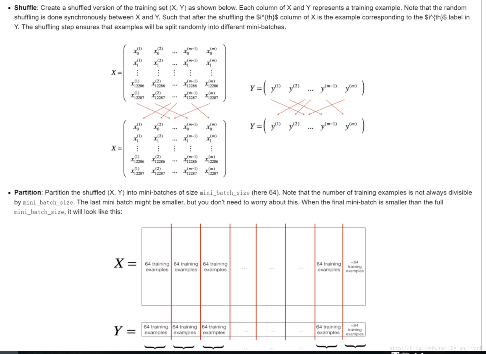
就在两步：

shuffle 置乱，让其尽量随机，这里需要注意的是要将对应的y一起之乱
partion 分割,其实就是选择一个batch size 这也是一个超参数，是需要调节的，andrew 在lecture中说最好取，16，64，128，…2的幂次，个人不知道是为什么，不过猜想和计算机的二进制有关，有很多硬件底层可以实现向量运算，而且长度是基于2的幂次的

代码

# GRADED FUNCTION: random_mini_batches

def random_mini_batches(X, Y, mini_batch_size = 64, seed = 0):
    """
    Creates a list of random minibatches from (X, Y)

    Arguments:
    X -- input data, of shape (input size, number of examples)
    Y -- true "label" vector (1 for blue dot / 0 for red dot), of shape (1, number of examples)
    mini_batch_size -- size of the mini-batches, integer

    Returns:
    mini_batches -- list of synchronous (mini_batch_X, mini_batch_Y)
    """

    np.random.seed(seed)            # To make your "random" minibatches the same as ours
    m = X.shape[1]                  # number of training examples
    mini_batches = []

    # Step 1: Shuffle (X, Y)
    permutation = list(np.random.permutation(m))
    shuffled_X = X[:, permutation]
    shuffled_Y = Y[:, permutation].reshape((1,m))

    # Step 2: Partition (shuffled_X, shuffled_Y). Minus the end case.
    num_complete_minibatches = math.floor(m/mini_batch_size) # number of mini batches of size mini_batch_size in your partitionning
    for k in range(0, num_complete_minibatches):
        ### START CODE HERE ### (approx. 2 lines)
        mini_batch_X = shuffled_X[:,k*mini_batch_size:(k+1)*mini_batch_size]
        mini_batch_Y = shuffled_Y[:,k*mini_batch_size:(k+1)*mini_batch_size]
        ### END CODE HERE ###
        mini_batch = (mini_batch_X, mini_batch_Y)
        mini_batches.append(mini_batch)

    # Handling the end case (last mini-batch < mini_batch_size)
    if m % mini_batch_size != 0:
        ### START CODE HERE ### (approx. 2 lines)
        mini_batch_X =shuffled_X[:,num_complete_minibatches*mini_batch_size:m] 
        mini_batch_Y = shuffled_Y[:,num_complete_minibatches*mini_batch_size:]
        ### END CODE HERE ###
        mini_batch = (mini_batch_X, mini_batch_Y)
        mini_batches.append(mini_batch)

    return mini_batches

注意

当batch size取0的时候，就是随机梯度下降，当取n(样本个数)为梯度下降，
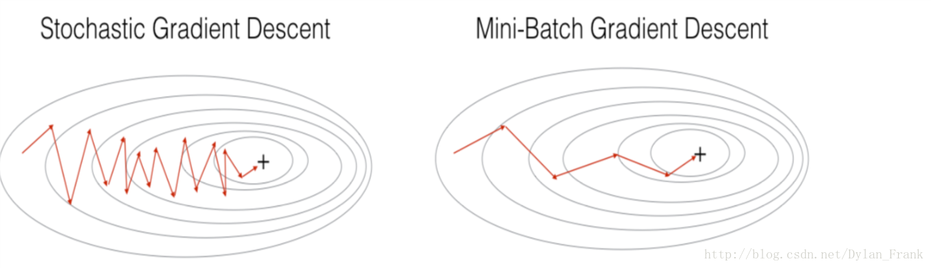
随机梯度下降和 mini-batch 梯度下降都是有波动的，不过mini-batch波动较小(这个问题后面会提出解决方法)
见下图：
当训练数据很大的时候小批量下降会有很大优势，比如最直接的一点是节省计算时间（计算所有样本的梯度时间花费更高）

momentum(动量)

这里写图片描述

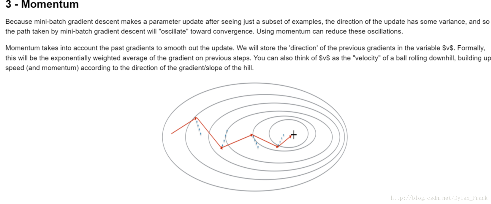
动量法试图解决小批量样本仅依赖原样本的子集带来的梯度波动问题，具体做法是它对过去的梯度加了一个指数权重，

{v d W [l] = β v d W [l] + (1 - β) d W [l] W [l] = W [l] - α v d W [l] (1)

$\begin{cases} v_{dW^{[l]}} = \beta v_{dW^{[l]}} + (1 - \beta) dW^{[l]} \\ W^{[l]} = W^{[l]} - \alpha v_{dW^{[l]}} \end{cases}\tag{1}$

{v d b [l] = β v d b [l] + (1 - β) d b [l] b [l] = b [l] - α v d b [l] (2)

$\begin{cases} v_{db^{[l]}} = \beta v_{db^{[l]}} + (1 - \beta) db^{[l]} \\ b^{[l]} = b^{[l]} - \alpha v_{db^{[l]}} \end{cases}\tag{2}$

其中 $v$ 一直在用以前的数据和现在的梯度的凸组合来更新自己，将 $v_0$ 设置为0，如果我门把 (1)式上面的式子一直推下去，会发现它对前面的梯度(passed)加了一个指数平均，来试图减缓这种波动.

code

# GRADED FUNCTION: update_parameters_with_momentum

def update_parameters_with_momentum(parameters, grads, v, beta, learning_rate):
    """
    Update parameters using Momentum

    Arguments:
    parameters -- python dictionary containing your parameters:
                    parameters['W' + str(l)] = Wl
                    parameters['b' + str(l)] = bl
    grads -- python dictionary containing your gradients for each parameters:
                    grads['dW' + str(l)] = dWl
                    grads['db' + str(l)] = dbl
    v -- python dictionary containing the current velocity:
                    v['dW' + str(l)] = ...
                    v['db' + str(l)] = ...
    beta -- the momentum hyperparameter, scalar
    learning_rate -- the learning rate, scalar

    Returns:
    parameters -- python dictionary containing your updated parameters 
    v -- python dictionary containing your updated velocities
    """

    L = len(parameters) // 2 # number of layers in the neural networks

    # Momentum update for each parameter
    for l in range(L):

        ### START CODE HERE ### (approx. 4 lines)
        # compute velocities
        v["dW" + str(l+1)] = beta*v["dW" + str(l+1)]+(1-beta)*grads['dW'+str(l+1)]
        v["db" + str(l+1)] = beta*v['db'+str(l+1)] + (1-beta)*grads['db'+str(l+1)]
        # update parameters
        parameters["W" + str(l+1)] =parameters["W" + str(l+1)] -learning_rate*v['dW'+str(l+1)] 
        parameters["b" + str(l+1)] =parameters["b" + str(l+1)] -learning_rate*v['db'+str(l+1)] 
        ### END CODE HERE ###

    return parameters, v

Adam

这是一种结合了RMSprop和动量的算法，它计算了梯度的平方的指数加权平均，它的更新规则如下

⎧ ⎩ ⎨ ⎪ ⎪ ⎪ ⎪ ⎪ ⎪ ⎪ ⎪ ⎪ ⎪ ⎪ ⎪ ⎪ ⎪ ⎪ ⎪ ⎪ ⎪ ⎪ ⎪ ⎪ ⎪ ⎪ ⎪ ⎪ ⎪ v d W [l] = β 1 v d W [l] + (1 - β 1) \partial J \partial W [ l ] v c o r r e c t e d d W [l] = v d W [ l ] 1 - ( β 1 ) t s d W [l] = β 2 s d W [l] + (1 - β 2) (\partial J \partial W [ l ]) 2 s c o r r e c t e d d W [l] = s d W [ l ] 1 - ( β 1 ) t W [l] = W [l] - α v c o r r e c t e d d W [ l ] s c o r r e c t e d d W [ l ] \sqrt + ε

$\begin{cases} v_{dW^{[l]}} = \beta_1 v_{dW^{[l]}} + (1 - \beta_1) \frac{\partial \mathcal{J} }{ \partial W^{[l]} } \\ v^{corrected}_{dW^{[l]}} = \frac{v_{dW^{[l]}}}{1 - (\beta_1)^t} \\ s_{dW^{[l]}} = \beta_2 s_{dW^{[l]}} + (1 - \beta_2) (\frac{\partial \mathcal{J} }{\partial W^{[l]} })^2 \\ s^{corrected}_{dW^{[l]}} = \frac{s_{dW^{[l]}}}{1 - (\beta_1)^t} \\ W^{[l]} = W^{[l]} - \alpha \frac{v^{corrected}_{dW^{[l]}}}{\sqrt{s^{corrected}_{dW^{[l]}}} + \varepsilon} \end{cases}$

其中 $\beta_1，\beta_2$ 是超参数，下图给出了建议值
《deeplearning》

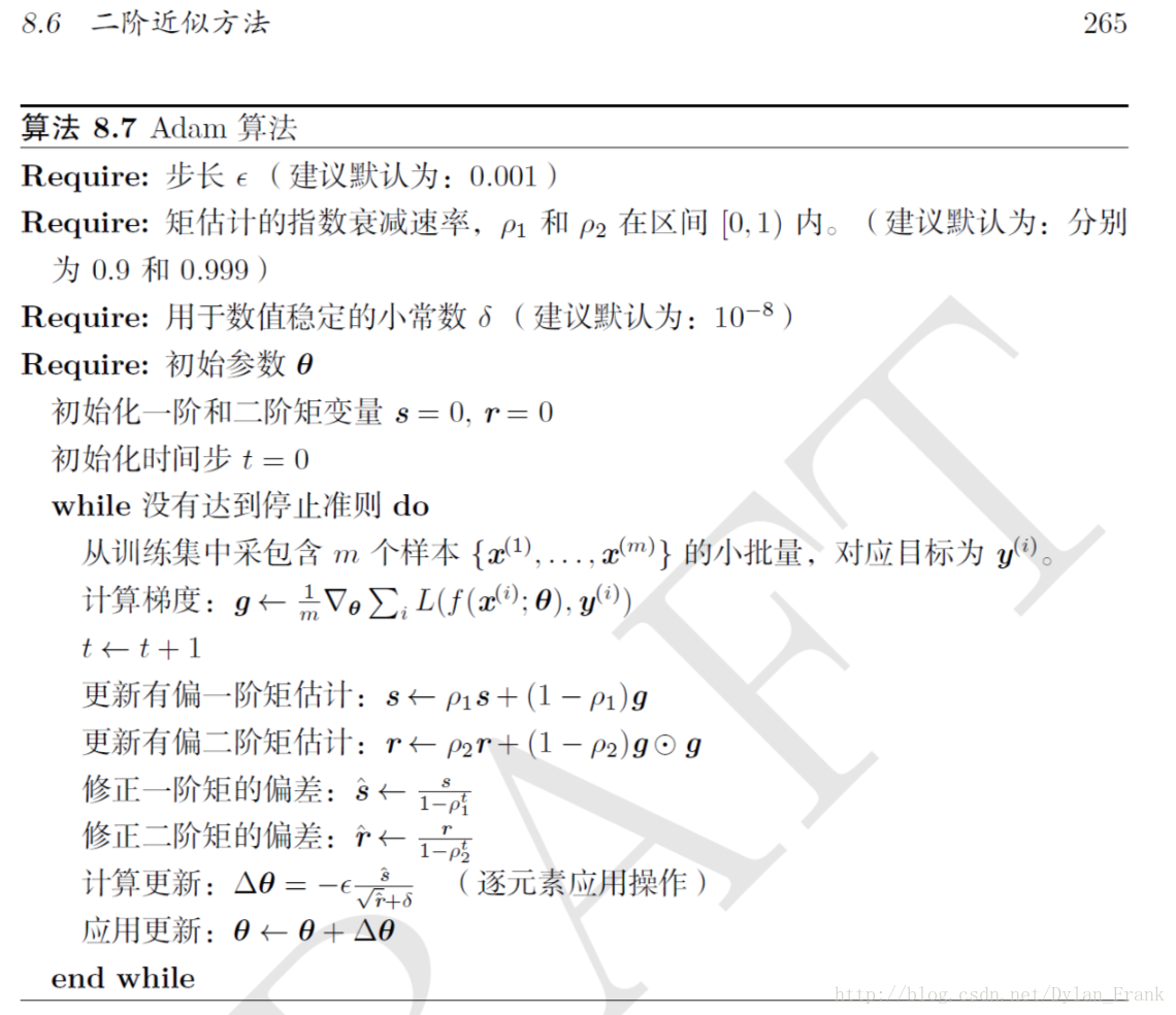
如果我们把他们的梯度提出来可以将这种算法视为学习速率的自适应(见《deeplearning》)

code

# GRADED FUNCTION: update_parameters_with_adam

def update_parameters_with_adam(parameters, grads, v, s, t, learning_rate = 0.01,
                                beta1 = 0.9, beta2 = 0.999,  epsilon = 1e-8):
    """
    Update parameters using Adam

    Arguments:
    parameters -- python dictionary containing your parameters:
                    parameters['W' + str(l)] = Wl
                    parameters['b' + str(l)] = bl
    grads -- python dictionary containing your gradients for each parameters:
                    grads['dW' + str(l)] = dWl
                    grads['db' + str(l)] = dbl
    v -- Adam variable, moving average of the first gradient, python dictionary
    s -- Adam variable, moving average of the squared gradient, python dictionary
    learning_rate -- the learning rate, scalar.
    beta1 -- Exponential decay hyperparameter for the first moment estimates 
    beta2 -- Exponential decay hyperparameter for the second moment estimates 
    epsilon -- hyperparameter preventing division by zero in Adam updates

    Returns:
    parameters -- python dictionary containing your updated parameters 
    v -- Adam variable, moving average of the first gradient, python dictionary
    s -- Adam variable, moving average of the squared gradient, python dictionary
    """

    L = len(parameters) // 2                 # number of layers in the neural networks
    v_corrected = {}                         # Initializing first moment estimate, python dictionary
    s_corrected = {}                         # Initializing second moment estimate, python dictionary

    # Perform Adam update on all parameters
    for l in range(L):
        # Moving average of the gradients. Inputs: "v, grads, beta1". Output: "v".
        ### START CODE HERE ### (approx. 2 lines)
        v["dW" + str(l+1)] = beta1*v["dW" + str(l+1)] + (1-beta1)*grads['dW'+str(l+1)]
        v["db" + str(l+1)] = beta1*v['db' + str(l+1)] + (1-beta1)*grads['db'+str(l+1)]
        ### END CODE HERE ###

        # Compute bias-corrected first moment estimate. Inputs: "v, beta1, t". Output: "v_corrected".
        ### START CODE HERE ### (approx. 2 lines)
        v_corrected["dW" + str(l+1)] = v['dW'+str(l+1)]/(1-beta1**t)
        v_corrected["db" + str(l+1)] = v['db'+str(l+1)]/(1-beta1**t)
        ### END CODE HERE ###

        # Moving average of the squared gradients. Inputs: "s, grads, beta2". Output: "s".
        ### START CODE HERE ### (approx. 2 lines)
        s["dW" + str(l+1)] = s["dW" + str(l+1)]*beta2 + (grads['dW'+str(l+1)]**2) * (1-beta2)
        s["db" + str(l+1)] = s['db' + str(l+1)] * beta2 + (grads['db' + str(l+1)] ** 2) * (1-beta2)
        ### END CODE HERE ###

        # Compute bias-corrected second raw moment estimate. Inputs: "s, beta2, t". Output: "s_corrected".
        ### START CODE HERE ### (approx. 2 lines)
        s_corrected["dW" + str(l+1)] =s['dW'+str(l+1)]/(1-beta2**t) 
        s_corrected["db" + str(l+1)] = s['db'+str(l+1)]/(1-beta2**t)
        ### END CODE HERE ###

        # Update parameters. Inputs: "parameters, learning_rate, v_corrected, s_corrected, epsilon". Output: "parameters".
        ### START CODE HERE ### (approx. 2 lines)
        parameters["W" + str(l+1)] =parameters["W" + str(l+1)] -learning_rate*v_corrected['dW'+str(l+1)]/(np.sqrt(s['dW'+str(l+1)])+epsilon) 
        parameters["b" + str(l+1)] =parameters["b" + str(l+1)] - learning_rate*v_corrected['db'+str(l+1)]/(np.sqrt(s['db'+str(l+1)])+epsilon)
        ### END CODE HERE ###

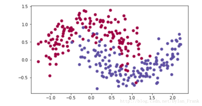
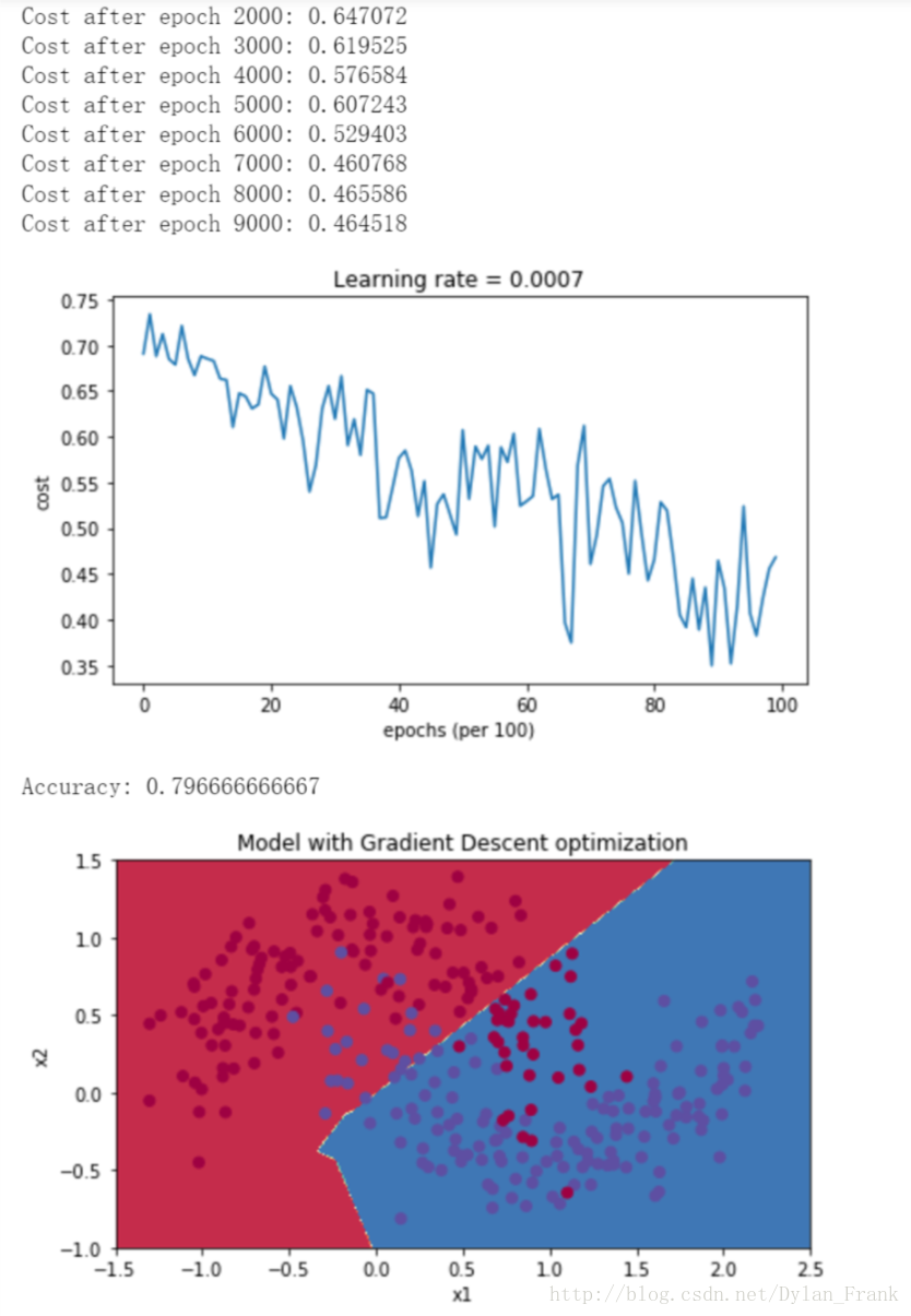
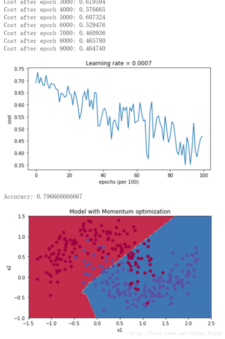
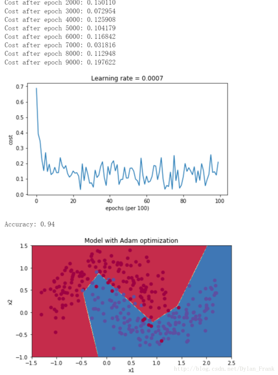
    return parameters, v, s

实验

以下图的数据集为例，给出3中算法实验结果
这里写图片描述

这里写图片描述

孤鸿子_

关注

0
点赞
踩
0

收藏

觉得还不错? 一键收藏
0
评论
deeplearning Note:Optimization

作者：dylanFrank(滔滔)这是deeplearning.ai的第二周，这周讲的是优化，这周其实有很多东西并不是很懂，个人结合了《deeplearning》这本书来自己理了一下，同时也本着迅速入门的想法就没有想那么多，现将其知识整理如下:mini-batch gradient descentmomentumRMSpropadamlearning rate decay本质上来说，
复制链接

扫一扫