


This series of articles are the study notes of " Machine Learning ", by Prof. Andrew Ng., Stanford University. This article is the notes of week 3, Solving the Problem of Overfitting. This article contains some topic about regularization, including overfitting, and how to implementation linear regression and logistic regression with regularization to addressing overfitting.
Solving the Problem of Overfitting
1. The problem of overfitting
By now, we've seen a couple different learning algorithms, linear regression and logistic regression. They work well for many problems, but when you apply them to certain machine learning applications, they can run into a problem called overfitting that can cause them to perform very poorly. In this section, we're going to explain what is this overfitting problem, and in the next few sections after this, we'll talk about a technique called regularization, that will allow us to ameliorate or to reduce this overfitting problem and get these learning algorithms to maybe work much better.
What is overfitting?
Example: Linear regression (housing prices)
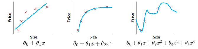
Underfit (High bias)
Just right
Overfitting:
but fail to generalize to new examples (predict prices on new examples).
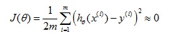
To recap a bit the problem of over fitting comes when if we have too many features, then to learn hypothesis may fit the training side very well. So, your cost function may actually be very close to zero or may be even zero exactly, but you may then end up with a curve like this that, you know tries too hard to fit the training set, so that it even fails to generalize to new examples and fails to predict prices on new examples as well, and here the term generalized refers to how well a hypothesis applies even to new examples.
Example: Logistic regression
A similar thing can apply to logistic regression as well. Here is a logistic regression example with two features x1 andx2.
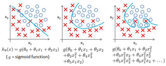
Underfit (High bias)
Just right
Overfitting (High variance)
finally, at the other extreme, if you were to fit a very high-order polynomial, if you were to generate lots of high-order polynomial terms of speeches, then, logistical regression may contort itself, may try really hard to find a decision boundary that fits your training data or go to great lengths to contort itself, to fit every single training example well.
This doesn't look like a very good hypothesis, for making predictions. And so, once again,this is an instance of overfitting and, of a hypothesis having high variance and, being unlikely to generalize well to new examples.
How to addressing overfitting?
lets talk about the problem of, if we think overfitting is occurring,what can we do to address it?
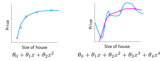
Plotting the hypothesis
In the previous examples, we had one or two dimensional data so, we could just plot the hypothesis and see what was going on and select the appropriate degree polynomial. And we could then use figures like these to select an appropriate degree polynomial. So plotting the hypothesis, could be one way to try to decide what degree polynomial to use.

But plotting the hypothesis doesn't always work. And, in fact more often we may have learning problems that where we just have a lot of features. And there is not just a matter of selecting what degree polynomial. And, in fact, when we have so many features, it also becomes much harder to plot the data and it becomes much harder to visualize it, to decide what features to keep or not.
Options to deal with overfitting:
1.Reduce number of features.
- ― Manually select which features to keep.
- ― Model selection algorithm(later in course).
2. Regularization.
- ― Keep all the features, but reduce magnitude/values of parametersθj.
- ― Works well when we have a lot of features, each of which contributes a bit to predicting y.
Try to reduce the number of features
Regularization
2. Cost Function
Intuition
Suppose we penalize and make θ3,θ4 really small.
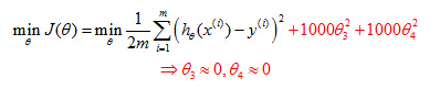
Penalizethe paramenters
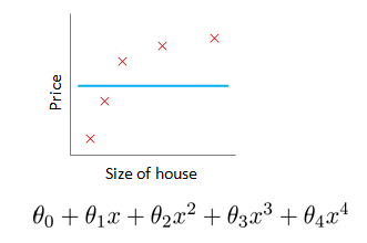
Consider the following, suppose we were to penalize, and, make the parametersθ3 and θ4 really small. Here is our optimization problem, where we minimize our usual squared error cause function. Let's say I take this objective and modify it and add to it, plus 1000θ3 squared, plus 1000 θ4 squared. 1000 I am just writing down as some huge number. Now, if we were to minimize this function, the only way to make this new cost function small is ifθ3 andθ4 are small. Because otherwise, if you have a thousand timesθ3, this new cost functions going to be big. So when we minimize this new function we are going to end up withθ3 close to 0 andθ4 close to 0, and as if we're getting rid of these two terms over there. Then we are being left with a quadratic function, and, so, we end up with a fit to the data, that's, you know, quadratic function plus maybe, tiny contributions from small terms, θ3 and θ4, that they may be very close to 0. And, so, we end up with essentially, a quadratic function, which is good. Because this is a much better hypothesis.
Get a simpler hypothesis
In this particular example, we looked at the effect of penalizing two of the parameter values being large. More generally, here is the idea behind regularization. The idea is that, if we have small values for the parameters, then, having small values for the parameters,will somehow, will usually correspond to having a simpler hypothesis. So, for our last example, we penalize justθ3 andθ4 and when both of these were close to zero, we will end up with a much simpler hypothesis that was essentially a quadratic function. But more broadly, if we penalize all the parameters usually that, we can think of that, as trying to give us a simpler hypothesis as well. Because when, these parameters areas close as you in this example, that gave us a quadratic function. But more generally, it is possible to show that having smaller values of the parameters corresponds to usually smoother functions as well for the simpler. And which are therefore, also, less prone to over fitting.
Regularization Cost Function
So we have a hundred or a hundred one parameters. And we don't know which ones to pick, we don't know which parameters to try to pick, to try to shrink. So, in regularization, what we're going to do, is take our cost function, here's my cost function for linear regression. And what I'm going to do is, modify this cost function to shrink all of my parameters, because, you know, I don't know which one or two to try to shrink. So I am going to modify my cost function to add a term at the end.
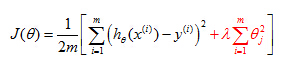
When I add an extra regularization term at the end to shrink every single parameter and so this term we tend to shrink all of my parameters theta 1, theta 2, theta 3 up to theta 100. By the way, by convention the summation here starts from one so I am not actually going penalize theta zero being large. That sort of the convention that, the sum I equals one through N, rather than I equals zero through N. But in practice, it makes very little difference, and, whether you include, you know, theta zero or not, in practice, make very little difference to the results. But by convention, usually, we regularize only theta through theta 100.
Choose there gularization parameterλ
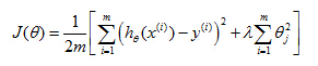
Here's J(θ) where, this term on the right is a regularization term andλhere is called the regularization parameter and what lambda does, is it controls a trade off between two different goals.
The first goal, capture it by the first goal objective, is that we would like to train, is that we would like to fit the training data well.
The second goalis, we want to keep the parameters small, and that's captured by the second term, by there regularization objective. And by there regularization term. And what lambda, the regularization parameter does is the controls the trade of between these two goals, between the goal of fitting the training set well and the goal of keeping the parameter plan small and therefore keeping the hypothesis relatively simple to avoid overfitting.
What if λ is set toan extremely large value (perhaps for too large for our problem, sayλ=1010)?
- Algorithm works fine; setting λ to be very large can’t hurt it
- Algorithm fails to eliminate overfitting.
- Algorithm results in underfitting. (Fails to fit even training data well).
- Gradient descent will fail to converge.
θ1≈0, θ2≈0, θ3≈0,θ4≈0,
hθ(x)=θ0


 5324
5324

 被折叠的 条评论
为什么被折叠?
被折叠的 条评论
为什么被折叠?
 到【灌水乐园】发言


