


 本文详细介绍了自适应直方图均衡化(AHE)和限制对比度自适应直方图均衡(CLAHE)算法。AHE用于提升图像对比度,但可能放大噪声,而CLAHE通过对比度限幅解决了这一问题。文章讨论了CLAHE的重分布和插值过程,以及如何通过插值提高算法效率。同时,还提供了matlab和c源码供参考。
1 自适应直方图均衡化(AHE)
自适应直方图均衡化(AHE)用来提升图像的对比度的一种计算机图像处理技术。和普通的直方图均衡算法不同,AHE算法通过计算图像的局部直方图,然后重新分布亮度来来改变图像对比度。因此,该算法更适合于改进图像的局部对比度以及获得更多的图像细节。但是,AHE有过度放大图像中相同区域的噪音的问题,另外一种自适应的直方图均衡算法即限制对比度直方图均衡(CLAHE)算法能有限地限制这种不利的放大。
普通的直方图均衡算法对于整幅图像的像素使用相同的直方图变换,对于那些像素值分布比较均衡的图像来说,算法的效果很好。然而,如果图像中包括明显比图像其它区域暗或者亮的部分,在这些部分的对比度将得不到有效的增强。
AHE算法通过对局部区域执行响应的直方图均衡来改变上述问题。该算法首先被开发出来适用于改进航天器驾驶舱的显示效果。其最简单的形式,就是每个像素通过其周边一个矩形范围内的像素的直方图进行均衡化。均衡的方式则完全同普通的均衡化算法:变换函数同像素周边的累积直方图函数(CDF)成比例。
图像边缘的像素需要特殊处理,因为边缘像素的领域不完全在图像内部。这个通过镜像图像边缘的行像素或列像素来解决。直接复制边缘的像素进行扩充是不合适的。因为这会导致带有剑锋的领域直方图。
2 限制对比度自适应直方图均衡(CLAHE)
2.1 重分布
CLAHE同普通的自适应直方图均衡不同的地方主要是其对比度限幅。这个特性也可以应用到全局直方图均衡化中,即构成所谓的限制对比度直方图均衡(CLHE),但这在实际中很少使用。在CLAHE中,对于每个小区域都必须使用对比度限幅。CLAHE主要是用来克服AHE的过度放大噪音的问题。 这主要是通过限制AHE算法的对比提高程度来达到的。在指定的像素值周边的对比度放大主要是由变换函数的斜度决定的。这个斜度和领域的累积直方图的斜度成比例。CLAHE通过在计算CDF前用预先定义的阈值来裁剪直方图以达到限制放大幅度的目的。这限制了CDF的斜度因此,也限制了变换函数的斜度。直方图被裁剪的值,也就是所谓的裁剪限幅,取决于直方图的分布因此也取决于领域大小的取值。通常,直接忽略掉那些超出直方图裁剪限幅的部分是不好的,而应该将这些裁剪掉的部分均匀的分布到直方图的其他部分。如下图所示。
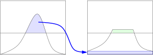
这个重分布的过程可能会导致那些倍裁剪掉的部分由重新超过了裁剪值(如上图的绿色部分所示)。如果效果不理想,可以重复进行这个过程直到超出部分已经变得微不足道了。
2.2 插值
如上所述,直接的自适应直方图,不管是否带有对比度限制,都需要对图像中的每个像素计算器领域直方图以及对应的变换函数,这使得算法极其耗时。 而插值使得上述算法效率上有极大的提升,并且质量上没有下降。首先,将图像均匀分成等份矩形大小,如下图的右侧部分所示(8行8列64个块是常用的选择)。然后计算个块的直方图、CDF以及对应的变换函数。这个变换函数对于块的中心像素(下图左侧部分的黑色小方块)是完全符合原始定义的。而其他的像素通过哪些于其临近的四个块的变换函数插值获取。位于图中蓝色阴影部分的像素采用双线性查插值,而位于便于边缘的(绿色阴影)部分采用线性插值,角点处(红色阴影处)直接使用块所在的变换函数。
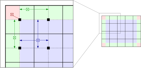
插值过程极大降低了变换函数需要计算的次数,只是增加了一些双线性插值的计算量。
3 源码
3.1 matlab源码
function out = adapthisteq(varargin)
%ADAPTHISTEQ Contrast-limited Adaptive Histogram Equalization (CLAHE).
%   ADAPTHISTEQ enhances the contrast of images by transforming the
%   values in the intensity image I.  Unlike HISTEQ, it operates on small
%   data regions (tiles), rather than the entire image. Each tile's
%   contrast is enhanced, so that the histogram of the output region
%   approximately matches the specified histogram. The neighboring tiles
%   are then combined using bilinear interpolation in order to eliminate
%   artificially induced boundaries.  The contrast, especially
%   in homogeneous areas, can be limited in order to avoid amplifying the
%   noise which might be present in the image.
%
%   J = ADAPTHISTEQ(I) Performs CLAHE on the intensity image I.
%
%   J = ADAPTHISTEQ(I,PARAM1,VAL1,PARAM2,VAL2...) sets various parameters.
%   Parameter names can be abbreviated, and case does not matter. Each
%   string parameter is followed by a value as indicated below:
%
%   'NumTiles'     Two-element vector of positive integers: [M N].
%                  [M N] specifies the number of tile rows and
%                  columns.  Both M and N must be at least 2.
%                  The total number of image tiles is equal to M*N.
%
%                  Default: [8 8].
%
%   'ClipLimit'    Real scalar from 0 to 1.
%                  'ClipLimit' limits contrast enhancement. Higher numbers
%                  result in more contrast.
%
%                  Default: 0.01.
%
%   'NBins'        Positive integer scalar.
%                  Sets number of bins for the histogram used in building a
%                  contrast enhancing transformation. Higher values result
%                  in greater dynamic range at the cost of slower processing
%                  speed.
%
%                  Default: 256.
%
%   'Range'        One of the strings: 'original' or 'full'.
%                  Controls the range of the output image data. If 'Range'
%                  is set to 'original', the range is limited to
%                  [min(I(:)) max(I(:))]. Otherwise, by default, or when
%                  'Range' is set to 'full', the full range of the output
%                  image class is used (e.g. [0 255] for uint8).
%
%                  Default: 'full'.
%
%   'Distribution' Distribution can be one of three strings: 'uniform',
%                  'rayleigh', 'exponential'.
%                  Sets desired histogram shape for the image tiles, by
%                  specifying a distribution type.
%
%                  Default: 'uniform'.
%
%   'Alpha'        Nonnegative real scalar.
%                  'Alpha' is a distribution parameter, which can be supplied
%                  when 'Dist' is set to either 'rayleigh' or 'exponential'.
%
%                  Default: 0.4.
%
%   Notes
%   -----
%   - 'NumTiles' specify the number of rectangular contextual regions (tiles)
%     into which the image is divided. The contrast transform function is
%     calculated for each of these regions individually. The optimal number of
%     tiles depends on the type of the input image, and it is best determined
%     through experimentation.
%
%   - The 'ClipLimit' is a contrast factor that prevents over-saturation of the
%     image specifically in homogeneous areas.  These areas are characterized
%     by a high peak in the histogram of the particular image tile due to many
%     pixels falling inside the same gray level range. Without the clip limit,
%     the adaptive histogram equalization technique could produce results that,
%     in some cases, are worse than the original image.
%
%   - ADAPTHISTEQ can use Uniform, Rayleigh, or Exponential distribution as
%     the basis for creating the contrast transform function. The distribution
%     that should be used depends on the type of the input image.
%     For example, underwater imagery appears to look more natural when the
%     Rayleigh distribution is used.
%
%   Class Support
%   -------------
%   Intensity image I can be uint8, uint16, int16, double, or single.
%   The output image J has the same class as I.
%
%   Example 1
%   ---------
%   Apply Contrast-Limited Adaptive Histogram Equalization to an
%   image and display the results.
%
%      I = imread('tire.tif');
%      A = adapthisteq(I,'clipLimit',0.02,'Distribution','rayleigh');
%      figure, imshow(I);
%      figure, imshow(A);
%
%   Example 2
%   ---------
%
%   Apply Contrast-Limited Adaptive Histogram Equalization to a color
%   photograph.
%
%      [X MAP] = imread('shadow.tif');
%      RGB = ind2rgb(X,MAP); % convert indexed image to truecolor format
%      cform2lab = makecform('srgb2lab');
%      LAB = applycform(RGB, cform2lab); %convert image to L*a*b color space
%      L = LAB(:,:,1)/100; % scale the values to range from 0 to 1
%      LAB(:,:,1) = adapthisteq(L,'NumTiles',[8 8],'ClipLimit',0.005)*100;
%      cform2srgb = makecform('lab2srgb');
%      J = applycform(LAB, cform2srgb); %convert back to RGB
%      figure, imshow(RGB); %display the results
%      figure, imshow(J);
%
%   See also HISTEQ, IMHISTMATCH.

%   Copyright 1993-2014 The MathWorks, Inc.

%   References:
%      Karel Zuiderveld, "Contrast Limited Adaptive Histogram Equalization",
%      Graphics Gems IV, p. 474-485, code: p. 479-484
%
%      Hanumant Singh, Woods Hole Oceanographic Institution, personal
%      communication

%--------------------------- The algorithm ----------------------------------
%
%  1. Obtain all the inputs:
%    * image
%    * number of regions in row and column directions
%    * number of bins for the histograms used in building image transform
%      function (dynamic range)
%    * clip limit for contrast limiting (normalized from 0 to 1)
%    * other miscellaneous options
%  2. Pre-process the inputs:
%    * determine real clip limit from the normalized value
%    * if necessary, pad the image before splitting it into regions
%
最低0.47元/天 解锁文章


 806
806

 被折叠的 条评论
为什么被折叠?
被折叠的 条评论
为什么被折叠?
 到【灌水乐园】发言


