


26.1 Support Vector Regression (SVR) using linear and non-linear
kernels
"""
===================================================================
Support Vector Regression (SVR) using linear and non-linear kernels
支持向量回归SVR使用线性linear与非线性核polynomial、RBF kernels
===================================================================

Toy example of 1D regression using linear, polynomial and RBF kernels.

"""
print(__doc__) #打印文本脚本说明

import numpy as np
from sklearn.svm import SVR
import matplotlib.pyplot as plt

###############################################################################
# Generate sample data #人工生成数据点
X = np.sort(5 * np.random.rand(40, 1), axis=0) # np.random.rand()随机生成[0,1]的随机数,默认是行向量,指定axis=0为列向量
y1 = np.sin(X)
y = np.sin(X).ravel() #将列向量转化为行向量
# ravel说明Ref:
# https://docs.scipy.org/doc/numpy/reference/generated/numpy.ravel.html
# http://blog.csdn.net/lanchunhui/article/details/50354978
# http://old.sebug.net/paper/books/scipydoc/numpy_intro.html

###############################################################################
# Add noise to targets #增加噪音
y[::5] += 3 * (0.5 - np.random.rand(8))
###############################################################################
# Fit regression model #拟合回归模型
#构建模型,设置模型超参数C,gamma,degree
svr_rbf = SVR(kernel='rbf', C=1e3, gamma=0.1)
svr_lin = SVR(kernel='linear', C=1e3)
svr_poly = SVR(kernel='poly', C=1e3, degree=2)
#用.fit()方法进行拟合,用.predict()方法进行预测,并返回预测结果
y_rbf = svr_rbf.fit(X, y).predict(X)
y_lin = svr_lin.fit(X, y).predict(X)
y_poly = svr_poly.fit(X, y).predict(X)

###############################################################################
# look at the results #查看结果
lw = 2 #设置线宽
#绘制人工数据散点图
plt.scatter(X, y, color='darkorange', label='data')
plt.hold('on') #类似Matlab中的hold on,可在同一个图中绘制后续图形

#绘制拟合曲线
plt.plot(X, y_rbf, color='navy', lw=lw, label='RBF model') #设置label用于后续legend的显示
plt.plot(X, y_lin, color='c', lw=lw, label='Linear model')
plt.plot(X, y_poly, color='cornflowerblue', lw=lw, label='Polynomial model')

#设置相关显示
plt.xlabel('data')
plt.ylabel('target')
plt.title('Support Vector Regression')
plt.legend()
plt.show()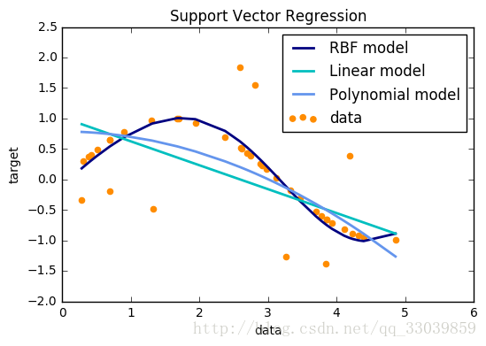
26.2 Non-linear SVM
"""
==============
Non-linear SVM
==============
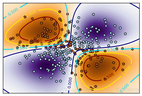
Perform binary classification using non-linear SVC with RBF kernel. The target to predict is a XOR of the inputs.
The color map illustrates the decision function learned by the SVC.
利用RBF核执行非线性SVC二分类,对于输入的XOR问题进行预测,颜色阐述了通过SVC学习得到的决策函数
Tips:如果a、b两个值不相同,则异或结果为1。如果a、b两个值相同,异或结果为0
"""
print(__doc__)
#导入需要调用的库
import numpy as np
import matplotlib.pyplot as plt
from sklearn import svm
#生成网格坐标点, xx,yy均是500x500的矩阵
xx, yy = np.meshgrid(np.linspace(-3, 3, 500),
np.linspace(-3, 3, 500))
#指定随机数种子
np.random.seed(0)
X = np.random.randn(300, 2)
Y = np.logical_xor(X[:, 0] > 0, X[:, 1] > 0)
# fit the model 拟合模型
#使用svm模块的NuSVC()函数,这个函数的功能是什么???
clf = svm.NuSVC()
clf.fit(X, Y)#利用fit训练模型clf
Z = clf.decision_function(np.c_[xx.ravel(), yy.ravel()])
Z = Z.reshape(xx.shape)
plt.imshow(Z, interpolation='nearest',
extent=(xx.min(), xx.max(), yy.min(), yy.max()), aspect='auto', #指定aspect=‘auto’自动改变图片的长宽比
origin='lower', cmap=plt.cm.PuOr_r) #cmap=plt.cm.安一次tabel键盘,可查看选择指定colormap的风格
contours = plt.contour(xx, yy, Z, levels=[0,0.5,1,1.5], linewidths=2,linetypes='--')#未指定xx,yy则无法绘制分类边界线
plt.clabel(contours, inline=1, fontsize=10) #绘制等高线上的标签
# 绘制散点图,分别取X的第一、第二列作为横纵坐标,s指定点的大小,c的值与Y的成正比,color的取值方式采用cmap=plt.cm.Paired)
plt.scatter(X[:, 0], X[:, 1], s=30, c=Y, cmap=plt.cm.Paired) #Y是False或True,cmap指定配对的颜色
plt.xticks(())
plt.yticks(())
plt.axis([-3, 3, -3, 3])
plt.show()
"""
# http://matplotlib.org/api/pyplot_api.html?highlight=matplot%20pyplot%20imshow#matplotlib.pyplot.imshow
# plot the decision function for each datapoint on the grid
# np.c_[ ]???按列将slice进行组合,同理np.c_[]将slice按行进行组合
# Ref:
# http://blog.csdn.net/crossky_jing/article/details/49466127
# https://docs.scipy.org/doc/numpy-1.6.0/reference/generated/numpy.c_.html
# ravel() 将500x500的矩阵逐行拼装称为一个行向量,np.c_[]将两个行向量进行拼装组合成一个250000x2的向量
# 利用训练好的模型进行分类,然后调用分类器集合的decision_function函数获得样本到超平面的距离。
# decision_function用法:Distance of the samples X to the separating hyperplane. 即样本点到超平面的距离。
# Z是一个n*1的矩阵(列向量),记录了n个样本距离超平面的距离。
#1
interpolation extent origin这三个参数是干嘛用的?
interpolation='nearest' simply display the image without try to interpolate betwen pixels
if the display resolution is not the same as the image resolution (which is most often the case).
It will results in an image in which is image pixel is displayed as a square of multiple display pixels.
#2
interpolation='nearest'即选取最近的像素点作为插值值,不再单独计算
#3
extent图像显示的范围,未设置的话,则坐标轴上的刻度变成矩阵的数目
http://matplotlib.org/api/pyplot_api.html?highlight=matplotlib%20pyplot%20cm#matplotlib.pyplot.set_cmap
contour(X,Y,Z): , X,Y specify the (x, y) coordinates of the surface
一共有500个数据点,则需要500个(x,y)
levels: [level0, level1, ..., leveln]
A list of floating point numbers indicating the level curves to draw, in increasing order;
e.g., to draw just the zero contour pass levels=[0]
"""
- 矩阵绘制及参数levels,origin设置与效果
levels: 对应plt.contour(),显示轮廓线
origin: 对应plt.imshow(),决定图像原点与矩阵原点是否重合,即图像的方向
plt.matshow(A): 绘制矩阵,将矩阵用图像显示
# 绘制矩阵Z
plt.matshow(xx)
plt.matshow(yy)
plt.matshow(Z)
plt.show()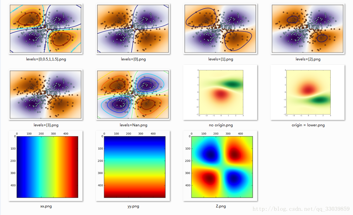


 2万+
2万+


 被折叠的 条评论
为什么被折叠?
被折叠的 条评论
为什么被折叠?
 到【灌水乐园】发言


