


stats中的optim函数是解决优化问题的一个简易的方法。
Univariate Optimization
- 1
- 2
- 3
- 1
- 2
- 3
General Optimization
optim函数包含了几种不同的算法。
算法的选择依赖于求解导数的难易程度,通常最好提供原函数的导数。
在求解之前,一般需要scale。
可以尝试用不同的方法求解同样的问题。
Nelder-Mead method
optim默认的方法。
又称下山单纯形法,可做非线性函数的极值以及曲线拟合。
其主要思想是:
在n维空间构建(n+1)顶点的多面体,通过reflection,expansion,contraction,来逐步逼近最佳点
x∗
。
特点是:
1. 不适用函数的导数信息
2. 对不可导函数适用
3. 可能很慢
BFGS method
属于quasi-Newton方法。
首先,简单介绍牛顿法:
牛顿法基于目标函数的二阶导数(海森矩阵),收敛速度快,迭代次数少,尤其在最优值附近,收敛速度是二次的。
缺点是:海森矩阵稠密时,每次迭代计算量交大,且每次都会重新计算目标函数的海森矩阵的逆。这样以来,问题规模大时,其计算量以及存储空间都很大。
拟牛顿法是在牛顿法基础上的改进,其引入了海森矩阵的近似矩阵,避免了每次迭代都需要计算海森矩阵的逆,其收敛速度介于梯度下降和牛顿法之间,属于超线性。
同时,牛顿法在每次迭代时不能保证海森矩阵总是正定的,一旦其不是正定,优化方向就会跑偏,从而使牛顿法失效,也证明了牛顿法的鲁棒性较差。
拟牛顿法利用海森矩阵的逆矩阵代替海森矩阵,虽然每次迭代不一定保证最优化的方向,但是近似矩阵始终正定,因此算法总是朝着最优值搜索。
注意:
1. 使用函数导数信息,通过人工提供或者有限微分
2. 高维的数据存储会很大
CG method
一种共轭梯度法(conjugate gradient),选择连续的、与椭圆轴线相仿的路径。
特点:
1. 不存储海森矩阵
2. 三种不同的路径搜索方法
3. 与BFGS相比,较差的鲁棒性
4. 使用函数导数信息
L-BFGS-B method
A limited memory version of BFGS
特点:
1. 不存储海森矩阵,只有一个对海森矩阵大小受限的更新步骤。
2. 使用导数信息
3. 可以把解决方法限制到box里,是optim中仅有的方法。
SANN method
模拟退火法(simulated annealing)的变种。
特点:
1. 随机算法
2. 接受以正概率提升目标的改变
3. 不使用导数信息
4. 收敛很慢,但是找到一个good solution很快
Brent method
An interface to optimize
特点:
1. 仅适用于一维问题
2. 可以在其他函数中包含
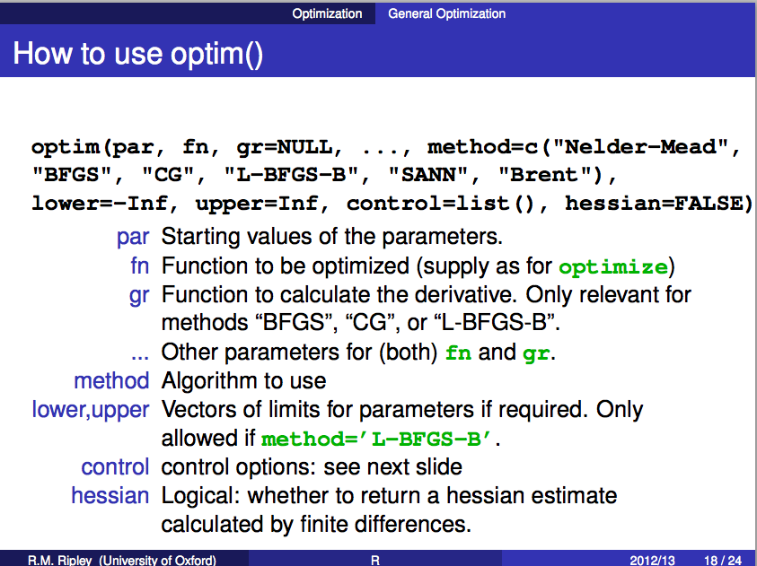
How to use
optim
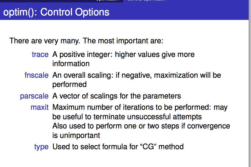
control options
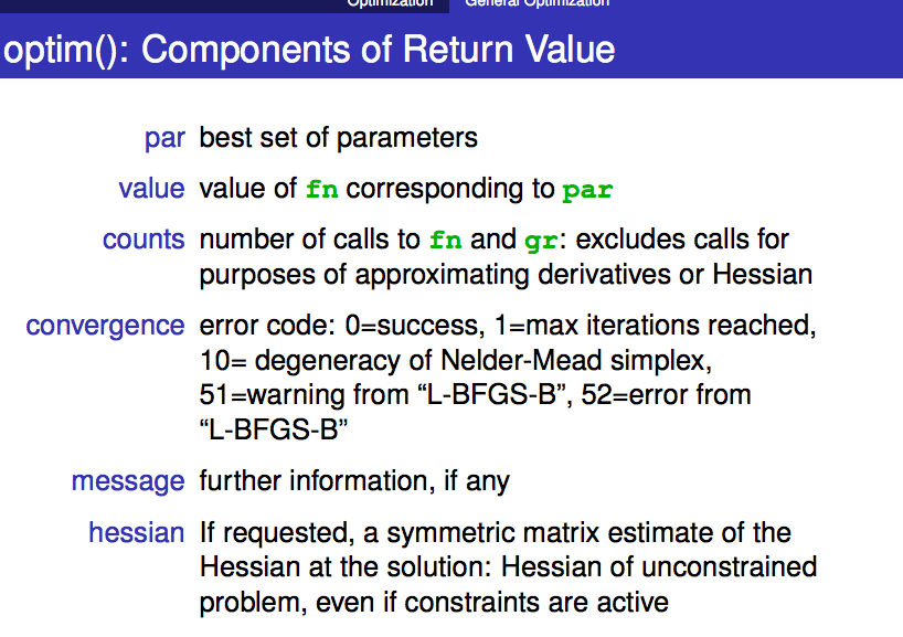
components of returned value
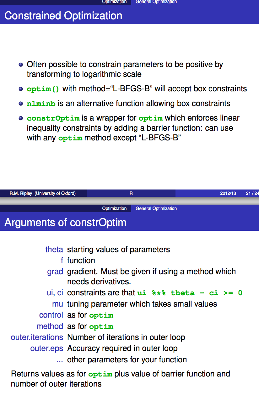
constrained optimization
Exampels
One Dimensional Ex1
假定
其导数为
- 1
- 2
- 3
- 4
- 5
- 6
- 7
- 8
- 9
- 10
- 11
- 12
- 13
- 14
- 15
- 16
- 1
- 2
- 3
- 4
- 5
- 6
- 7
- 8
- 9
- 10
- 11
- 12
- 13
- 14
- 15
- 16
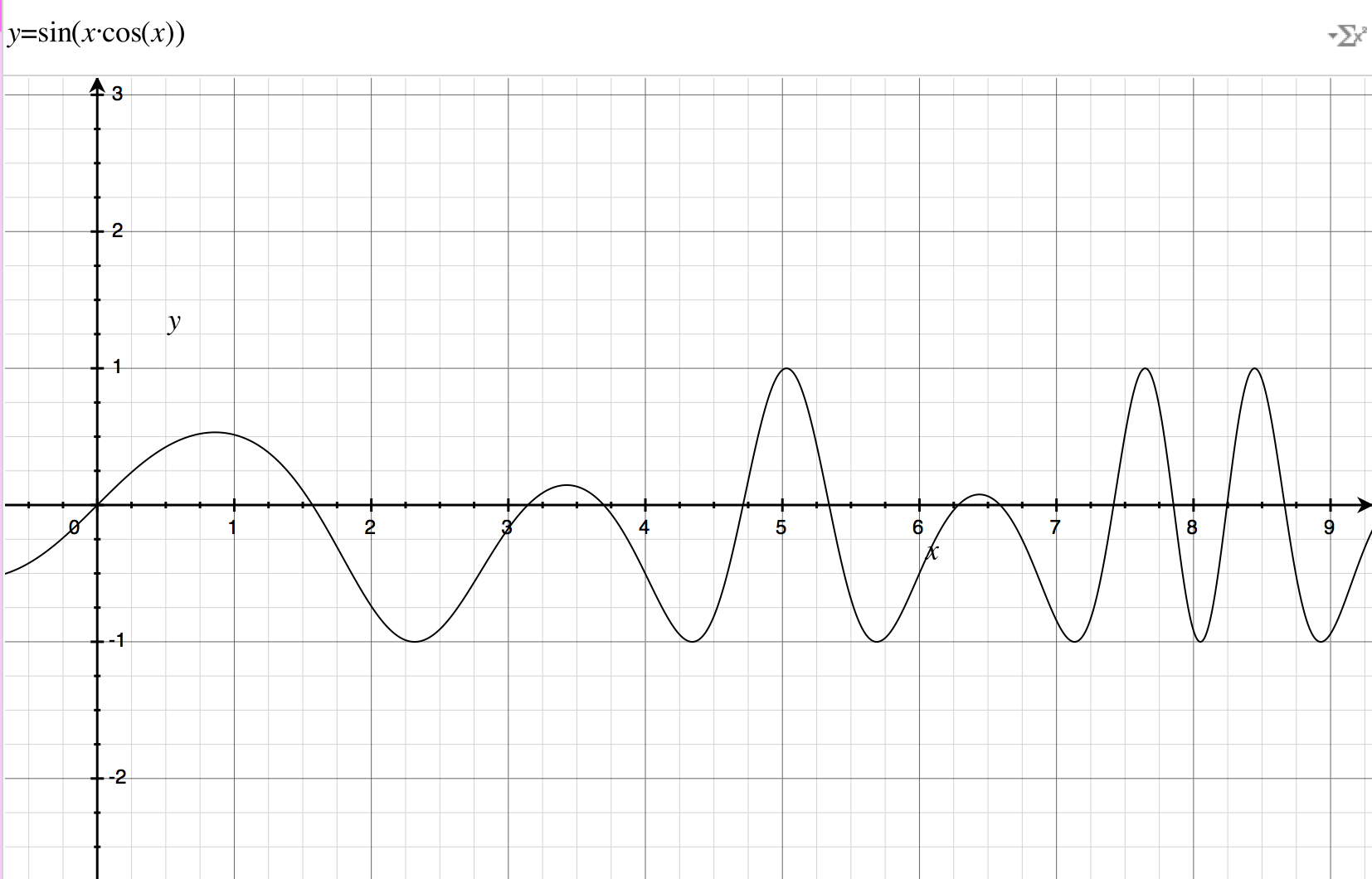
One Dimensional Ex2
假定
- 1
- 2
- 3
- 4
- 5
- 6
- 7
- 1
- 2
- 3
- 4
- 5
- 6
- 7
Two Dimensional Ex3
Rosenbrock function:
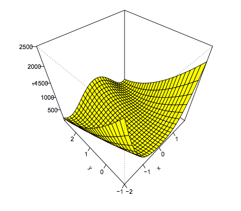
This function is strictly positive, but is 0 when y = x^2, and x = 1, so (1, 1) is a minimum.
Let’s see if optim can figure this out. When using optim for multidimensional optimization, the input in your function definition must be a single vector.
- 1
- 2
- 3
- 4
- 5
- 6
- 7
- 8
- 9
- 10
- 11
- 1
- 2
- 3
- 4
- 5
- 6
- 7
- 8
- 9
- 10
- 11
Two Dimensional Ex4
Himmelblau’s function:
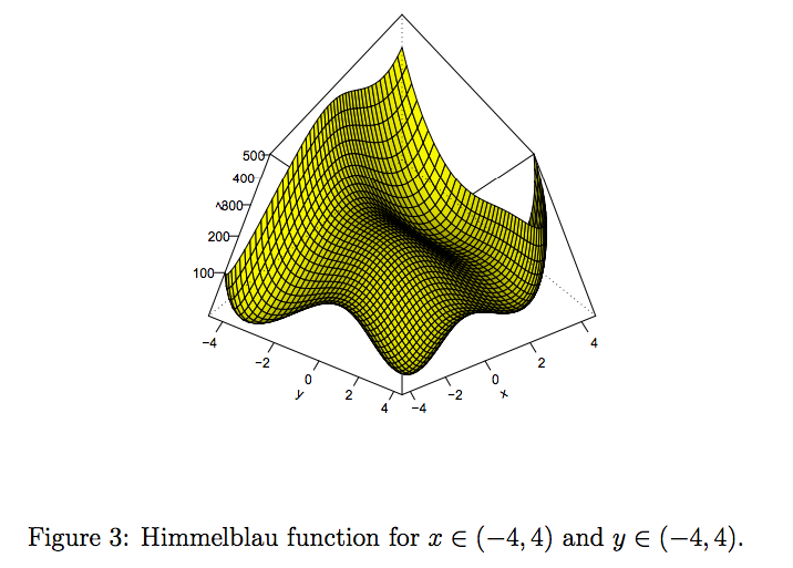
There appear to be four “bumps” that look like minimums in the realm of (-4,-4), (2,-2),(2,2) and (-4,4).
Again this function is strictly positive so the function is minimized when x^2 + y − 11 = 0 and x + y^2 − 7 = 0.
- 1
- 2
- 3
- 4
- 5
- 6
- 7
- 8
- 9
- 10
- 11
- 12
- 13
- 14
- 1
- 2
- 3
- 4
- 5
- 6
- 7
- 8
- 9
- 10
- 11
- 12
- 13
- 14
Fit a probit regression model
pass
Minimise residual sum of squares
- 1
- 2
- 3
- 4
- 5
- 6
- 7
- 8
- 9
- 10
- 11
- 12
- 13
- 14
- 15
- 16
- 17
- 18
- 19
- 20
- 21
- 22
- 23
- 1
- 2
- 3
- 4
- 5
- 6
- 7
- 8
- 9
- 10
- 11
- 12
- 13
- 14
- 15
- 16
- 17
- 18
- 19
- 20
- 21
- 22
- 23
Maximum likelihood
To fit a Poisson distribution to x I don’t minimise the residual sum of squares, instead I maximise the likelihood for the chosen parameter lambda.


 1619
1619

 被折叠的 条评论
为什么被折叠?
被折叠的 条评论
为什么被折叠?
 到【灌水乐园】发言


