[Coursera机器学习]Logistic Regression WEEK3编程作业

1.1 Visualizing the data

To help you get more familiar with plotting, we have left plotData.m empty so you can try to implement it yourself. However, this is an optional(ungraded) exercise. We also provide our implementation below so you can copy it or refer to it.

% Find Indices of Positive and Negative Examples
pos = find(y==1); neg = find(y == 0);
% Plot Examples
plot(X(pos, 1), X(pos, 2), 'k+','LineWidth', 2, ...
'MarkerSize', 7);
plot(X(neg, 1), X(neg, 2), 'ko', 'MarkerFaceColor', 'y', ...
'MarkerSize', 7);

1.2.1 Warmup exercise: sigmoid function

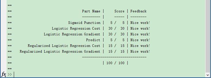
Your rst step is to implement this function in sigmoid.m so it can be called by the rest of your program. When you are nished, try testing a few values by calling sigmoid(x) at the Octave/MATLAB command line.

$g(z) = \frac{1}{1 + e^{-z}}$

% ====================== YOUR CODE HERE ======================
% Instructions: Compute the sigmoid of each value of z (z can be a matrix,
%               vector or scalar).
g = 1 ./ (1 + exp(-z));

1.2.2 Cost function and gradient

Now you will implement the cost function and gradient for logistic regression.
Complete the code in costFunction.m to return the cost and gradient.
Recall that the cost function in logistic regression is:

$J(\theta ) = \frac{1}{m}\sum_{i=1}^{m}[-y^{(i)}log(h_{\theta }(x^{(i)})) - (1-y^{(i)})log(1 - h_{\theta }(x^{(i)}))]$

$\frac{\partial J(\theta )}{\partial \theta _{j}} = \frac{1}{m}\sum_{i=1}^{m}(h_{\theta }(x^{(i)}) - y^{(i)})x_{j}^{(i)}$

J = (1 / m) * (-y' * log(sigmoid(X * theta)) - (1-y)' * log(1 - sigmoid(X*theta)));
grad = (1 / m) * X' * (sigmoid(X * theta) - y);

1.2.4 Evaluating logistic regression

Another way to evaluate the quality of the parameters we have found is to see how well the learned model predicts on our training set. In this part, your task is to complete the code in predict.m. The predict functionwill produce “1” or “0” predictions given a dataset and a learned parameter vector $\theta$.

% ====================== YOUR CODE HERE ======================
% Instructions: Complete the following code to make predictions using
%               your learned logistic regression parameters. 
%               You should set p to a vector of 0's and 1's
%
p = round( sigmoid(X * theta) )

2.3 Cost function and gradient

Now you will implement code to compute the cost function and gradient for regularized logistic regression. Complete the code in costFunctionReg.m to return the cost and gradient.
Recall that the regularized cost function in logistic regression is:

$J(\theta ) = \frac{1}{m}\sum_{i=1}^{m}[-y^{(i)}log(h_{\theta }(x^{(i)})) - (1-y^{(i)})log(1 - h_{\theta }(x^{(i)}))] + \frac{\lambda }{2m}\sum_{j=1}^{n}\theta _{j}^{2}$

$\frac{\partial J(\theta )}{\partial \theta _{0}} = \frac{1}{m}\sum_{i=1}^{m}(h_{\theta }(x^{(i)}) - y^{(i)})x_{j}^{(i)}$           for j = 0

$\frac{\partial J(\theta )}{\partial \theta _{j}} = \frac{1}{m}\sum_{i=1}^{m}(h_{\theta }(x^{(i)}) - y^{(i)})x_{j}^{(i)}+\frac{\lambda }{m}\theta _{j}$          for j $\geq$ 1

% ====================== YOUR CODE HERE ======================
% Instructions: Compute the cost of a particular choice of theta.
%               You should set J to the cost.
%               Compute the partial derivatives and set grad to the partial
%               derivatives of the cost w.r.t. each parameter in theta

n = size(theta, 1);
% You should not regularize theta(1)
theta_reg = [0; theta(2:n)];
J = (1 / m) * (-y' * log(sigmoid(X * theta)) - (1-y)' * log(1 - sigmoid(X*theta))) + lambda * (1 / (2 * m)) * sum(theta_reg .^ 2);
grad = (1 / m) * X' * (sigmoid(X * theta) - y) + lambda * (1 / m) * theta_reg;