


最小二乘法(又称最小平方法)是一种数学优化技术。它通过最小化误差的平方和寻找数据的最佳函数匹配。
利用最小二乘法可以简便地求得未知的数据,并使得这些求得的数据与实际数据之间误差的平方和为最小。
最小二乘法还可用于曲线拟合。
其他一些优化问题也可通过最小化能量或最大化熵用最小二乘法来表达。
示例[编辑]

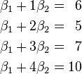
某次实验得到了四个数据点  :
: 、
、 、
、 、
、 (右图中红色的点)。我们希望找出一条和这四个点最匹配的直线
 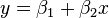 ,即找出在某种“最佳情况”下能够大致符合如下超定线性方程组的
  和
和  :
:
最小二乘法采用的手段是尽量使得等号两边的方差最小,也就是找出这个函数的最小值:
![\begin{align}S(\beta_1, \beta_2) = &\left[6-(\beta_1+1\beta_2)\right]^2+\left[5-(\beta_1+2\beta_2) \right]^2 \\&+\left[7-(\beta_1 + 3\beta_2)\right]^2+\left[10-(\beta_1 + 4\beta_2)\right]^2.\\\end{align}](http://upload.wikimedia.org/math/a/2/1/a21abd8e36caa43fcfd6dedbbaac4af1.png)
最小值可以通过对  分别求 和 的偏导数,然后使它们等于零得到。
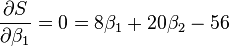
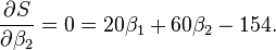
如此就得到了一个只有两个未知数的方程组,很容易就可以解出:


也就是说直线  是最佳的。
是最佳的。
简介[编辑]

1801年,意大利天文学家朱赛普·皮亚齐发现了第一颗小行星谷神星。经过40天的跟踪观测后,由于谷神星运行至太阳背后,使得皮亚齐失去了谷神星的位置。随后全世界的科学家利用皮亚齐的观测数据开始寻找谷神星,但是根据大多数人计算的结果来寻找谷神星都没有结果。时年24岁的高斯也计算了谷神星的轨道。奥地利天文学家海因里希·奥尔伯斯根据高斯计算出来的轨道重新发现了谷神星。
高斯使用的最小二乘法的方法发表于1809年他的著作《天体运动论》中,而法国科学家勒让德于1806年独立发现“最小二乘法”,但因不为时人所知而默默无闻。两人曾为谁最早创立最小二乘法原理发生争执。
1829年,高斯提供了最小二乘法的优化效果强于其他方法的证明,见高斯-马尔可夫定理。
方法[编辑]
人们对由某一变量 或多个变量
或多个变量 ……
…… 构成的相关变量
 感兴趣。如弹簧的形变与所用的力相关,一个企业的盈利与其营业额,投资收益和原始资本有关。为了得到这些变量同之间的关系,便用不相关变量去构建,使用如下函数模型
-
 ,
,
 个独立变量或
 个系数去拟和。
通常人们将一个可能的、对不相关变量t的构成都无困难的函数类型称作函数模型(如抛物线函数或指数函数)。参数b是为了使所选择的函数模型同观测值y相匹配。(如在测量弹簧形变时,必须将所用的力与弹簧的膨胀系数联系起来)。其目标是合适地选择参数,使函数模型最好的拟合观测值。一般情况下,观测值远多于所选择的参数。
其次的问题是怎样判断不同拟合的质量。高斯和勒让德的方法是,假设测量误差的平均值为0。令每一个测量误差对应一个变量并与其它测量误差不相关(随机无关)。人们假设,在测量误差中绝对不含系统误差,它们应该是纯偶然误差(有固定的变异数),围绕真值波动。除此之外,测量误差符合正态分布,这保证了偏差值在最后的结果y上忽略不计。
确定拟合的标准应该被重视,并小心选择,较大误差的测量值应被赋予较小的权。并建立如下规则:被选择的参数,应该使算出的函数曲线与观测值之差的平方和最小。用函数表示为:

用欧几里得度量表达为:

最小化问题的精度,依赖于所选择的函数模型。
线性函数模型[编辑]
典型的一类函数模型是线性函数模型。最简单的线性式是 ,写成矩阵式,为
直接给出该式的参数解:
-
 和
和

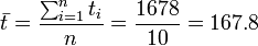
其中 ,为t值的算术平均值。也可解得如下形式:

简单线性模型 y = b0 + b1t 的例子[编辑]
随机选定10艘战舰,并分析它们的长度与宽度,寻找它们长度与宽度之间的关系。由下面的描点图可以直观地看出,一艘战舰的长度(t)与宽度(y)基本呈线性关系。散点图如下: 
以下图表列出了各战舰的数据,随后步骤是采用最小二乘法确定两变量间的线性关系。
| 编号 | 长度 (m) | 宽度 (m) | ti - t | yi - y | |||
|---|---|---|---|---|---|---|---|
| i | ti | yi | ti* | yi* | ti*yi* | ti*ti* | yi*yi* |
| 1 | 208 | 21.6 | 40.2 | 3.19 | 128.238 | 1616.04 | 10.1761 |
| 2 | 152 | 15.5 | -15.8 | -2.91 | 45.978 | 249.64 | 8.4681 |
| 3 | 113 | 10.4 | -54.8 | -8.01 | 438.948 | 3003.04 | 64.1601 |
| 4 | 227 | 31.0 | 59.2 | 12.59 | 745.328 | 3504.64 | 158.5081 |
| 5 | 137 | 13.0 | -30.8 | -5.41 | 166.628 | 948.64 | 29.2681 |
| 6 | 238 | 32.4 | 70.2 | 13.99 | 982.098 | 4928.04 | 195.7201 |
| 7 | 178 | 19.0 | 10.2 | 0.59 | 6.018 | 104.04 | 0.3481 |
| 8 | 104 | 10.4 | -63.8 | -8.01 | 511.038 | 4070.44 | 64.1601 |
| 9 | 191 | 19.0 | 23.2 | 0.59 | 13.688 | 538.24 | 0.3481 |
| 10 | 130 | 11.8 | -37.8 | -6.61 | 249.858 | 1428.84 | 43.6921 |
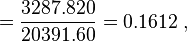
| 总和(Σ) | 1678 | 184.1 | 0.0 | 0.00 | 3287.820 | 20391.60 | 574.8490 |
仿照上面给出的例子
 并得到相应的
 .
.
然后确定b1

可以看出,战舰的长度每变化1m,相对应的宽度便要变化16cm。并由下式得到常数项b0:

在这里随机理论不加阐述。可以看出点的拟合非常好,长度和宽度的相关性大约为96.03%。 利用Matlab得到拟合直线: 
一般线性情况[编辑]
若含有更多不相关模型变量 ,可如组成线性函数的形式

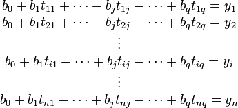
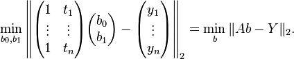
通常人们将tij记作数据矩阵 A,参数bj记做参数向量b,观测值yi记作Y,则线性方程组又可写成:
-
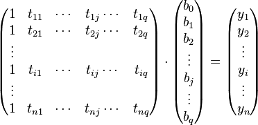 即
即

上述方程运用最小二乘法导出为线性平方差计算的形式为:
-
 。
。
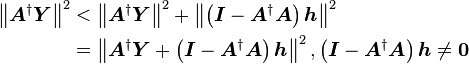
最小二乘法的解[编辑]

的特解为A的广义逆矩阵与Y的乘积,这同时也是二范数极小的解,其通解为特解加上A的零空间。证明如下:
先将Y拆成A的值域及其正交补两部分


所以 ,可得
,可得

故当且仅当 是
是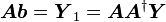 解时,即为最小二乘解,即
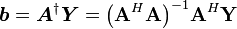 。
。
又因为

故 的通解为
的通解为

因为
所以 又是二范数极小的最小二乘解。
以上摘自WiKi百科
| Age (years) | DBH (inch) |
|---|---|
| 97 | 12.5 |
| 93 | 12.5 |
| 88 | 8.0 |
| 81 | 9.5 |
| 75 | 16.5 |
| 57 | 11.0 |
| 52 | 10.5 |
| 45 | 9.0 |
| 28 | 6.0 |
| 15 | 1.5 |
| 12 | 1.0 |
| 11 | 1.0 |
更多请看这里
| Curve Fitting, Regression |
 |
| Field data is often accompanied by noise. Even though all control parameters (independent variables) remain constant, the resultant outcomes (dependent variables) vary. A process of quantitatively estimating the trend of the outcomes, also known as regression or curve fitting, therefore becomes necessary. The curve fitting process fits equations of approximating curves to the raw field data. Nevertheless, for a given set of data, the fitting curves of a given type are generally NOT unique. Thus, a curve with a minimal deviation from all data points is desired. This best-fitting curve can be obtained by the method of least squares. |
| The Method of Least Squares |
|
| The method of least squares assumes that the best-fit curve of a given type is the curve that has the minimal sum of the deviations squared (least square error) from a given set of data. Suppose that the data points are 
|
 ,
,  , ...,
  where
where  is the independent variable and
  is the dependent variable. The fitting curve
  has the deviation (error)
 from each data point, i.e.,
  ,
,  , ...,
  . According to the method of least squares, the best fitting curve has the property that:
| Polynomials Least-Squares Fitting |
|
| Polynomials are one of the most commonly used types of curves in regression. The applications of the method of least squares curve fitting using polynomials are briefly discussed as follows. To obtain further information on a particular curve fitting, please click on the link at the end of each item. Or try the calculator on the right |
| The Least-Squares Line | ||
| ||
| The least-squares line uses a straight line
to approximate the given set of data, 
Please note that 
Expanding the above equations, we have: 
The unknown coefficients 
where |


 . The best fitting curve
  and
and  are unknown coefficients while all
  and
and  are given. To obtain the least square error, the unknown coefficients
  stands for
  .
.| The Least-Squares Parabola | ||
| ||
| The least-squares parabola uses a second degree curve
to approximate the given set of data, 
Please note that 
Expanding the above equations, we have 
The unknown coefficients |
 . The best fitting curve
  are unknown coefficients while all
 | The Least-Squares mth Degree Polynomials | ||
| ||
| When using an mth degree polynomial
to approximate the given set of data, 
Please note that 
Expanding the above equations, we have 
The unknown coefficients |
 , the best fitting curve
  ,
,  ,
,  , ..., and
  are unknown coefficients while all
 | Multiple Regression |
|
| Multiple regression estimates the outcomes (dependent variables) which may be affected by more than one control parameter (independent variables) or there may be more than one control parameter being changed at the same time. An example is the two independent variables For a given data set 
Please note that 
Expanding the above equations, we have 
The unknown coefficients |
 in the linear relationship case:
 ,
,  , ...,
  , where
  are given. To obtain the least square error, the unknown coefficients
Line of Best Fit(Least Square Method)
A line of best fit is a straight line that is the best approximation of the given set of data.
It is used to study the nature of the relation between two variables.
A line of best fit can be roughly determined using an eyeball method by drawing a straight line on a scatter plot so that the number of points above the line and below the line is about equal (and the line passes through as many points as possible).
A more accurate way of finding the line of best fit is the least square method .
Use the following steps to find the equation of line of best fit for a set of ordered pairs.
Step 1: Calculate the mean of the x-values and the mean of the y-values.
Step 2: Compute the sum of the squares of the x-values.
Step 3: Compute the sum of each x-value multiplied by its corresponding y-value.
Step 4: Calculate the slope of the line using the formula:
where n is the total number of data points.

Step 5: Compute the y-intercept of the line by using the formula:
where
are the mean of the x- and y-coordinates of the data points respectively.

Step 6: Use the slope and the y -intercept to form the equation of the line.
Example:
Use the least square method to determine the equation of line of best fit for the data. Then plot the line.

Solution:
Plot the points on a coordinate plane.

Calculate the means of the x-values and the y-values, the sum of squares of the x-values, and the sum of each x-value multiplied by its corresponding y-value.

Calculate the slope.

Calculate the y-intercept.
First, calculate the mean of the x-values and that of the y-values.

Use the formula to compute the y-intercept.

Use the slope and y-intercept to form the equation of the line of best fit.
The slope of the line is –1.1 and the y -intercept is 14.0.
Therefore, the equation is y = –1.1 x + 14.0.
Draw the line on the scatter plot.

最小二乘法在解决机器学习中的回归分析
最小二乘法的简单具体实现:
最基本的:
#include<iostream>
#include<conio.h>
#include<math.h>
using namespace std;
int main()
{
	int n,i,j;
	float a,a0,a1,x[10],f[10],sumx=0,sumy=0,sumxy=0,sumx2=0;
	cout<<"Enter no of sample points ? ";cin>>n;
	cout<<"Enter all sample points: "<<endl;
	for(i=0;i<n;i++)
	{
		cin>>x[i]>>f[i]; // read both (x,f(x))
		sumx+=x[i];
		sumy+=f[i];
		sumxy+=x[i]*f[i];
		sumx2+=x[i]*x[i];
	}
	cout<<"your sample x ? ";
	cin>>a;
	a0=(sumy*sumx2-sumx*sumxy)/(n*sumx2-sumx*sumx);
	a1=(n*sumxy-sumx*sumy)/(n*sumx2-sumx*sumx);
	cout<<"The coefficients are : "<<endl<<a0<<endl<<a1;
	cout<<endl<<"f("<<a<<"): "<<(a0+a1*a);
	getch();
	return 0;
}
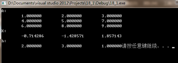
CvMat形式
#include<iostream>
#include <opencv2/opencv.hpp>
using namespace std;
using namespace cv;

void main()
{
	float   a[9]={1,2,3,4,5,7,6,8,9};
	float   b[3]={2,3,1};
	CvMat*   A   =   cvCreateMat(3,3,CV_32FC1);
	CvMat*   X   =   cvCreateMat(3,1,CV_32FC1);
	CvMat*   B   =   cvCreateMat(3,1,CV_32FC1);

	cvSetData(A,a,CV_AUTOSTEP);
	cvSetData(B,b,CV_AUTOSTEP);
	cvSolve(A,B,X,CV_LU);   //   solve (Ax=b) for x

	printf("A:");
	for(int i=0;i < 9; i++)
	{
		if(i%3==0) printf("\n");
		printf("\t%f",A->data.fl[i]);
	}

	printf("\nX:\n");
	for(int i = 0;i < 3; i++)
	{
		printf("\t%f",X->data.fl[i]);
	}

	printf("\nb:\n");
	for(int i=0;i<3;i++)
	{
		printf("\t%f",B->data.fl[i]);
	}
	system("pause");
} 
更详细的内容请看 这里


 1万+
1万+


 被折叠的 条评论
为什么被折叠?
被折叠的 条评论
为什么被折叠?
 到【灌水乐园】发言


