短期气候Python绘图——中国夏季降水分布以及环流异常分析

一、要求

掌握短期气候预测因子的分析和选择，加深对夏季降水分布、环流异常在短期气候预测中物理机制的认识 。

二、资料说明

（1）NCEP/NCAR 再分析资料1948－2012年1～12月的500百帕月平均高度场资料

网格距2.5°×2.5°,纬向格点数144，经向格点数73

范围（90°S-90°N,0-360°E)

网格距2.5°×2.5°,纬向格点数144，经向格点数73

资料为GRD格式，资料从南到北、自西向东排列，每月为一个记录，按年逐月排放。

（2）国家气候中心整编的6、7、8月降水量资料    （时间段：1951~2010年，资料的格式参见readme.txt文件）

（3）

1951~2010年雨型分类表

       1  0  0   一类雨型

       0  1  0   二类雨型

       0  0  1   三类雨型

三、方法介绍

(1)降水距平百分率：

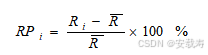
Ri某年夏季降水量

为1971-2000年夏季降水多年平均值   

(2)总体均值的t统计量：

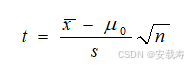
(3)总体均值的t统计量：

一、二、三类雨型的样本数分别为22、19和19。我们认为简单认为它们通过0.01显著性水平的t值分别为2.85，2.90，2.90，通过0.05显著性水平的t值都为2.09，2.11，2.11。

四、代码

（1）中国夏季三类雨型

import numpy as np
import pandas as pd
import matplotlib.pyplot as plt
import cartopy.crs as ccrs
import cartopy.feature as cfeature
import cartopy.mpl.ticker as cticker
import scipy.stats as stats
import xarray as xr
import geopandas as gpd
from scipy.interpolate import griddata
import salem
from cartopy.io.shapereader import Reader

def readdata(filename):
    data = []
    file1 = open(filename, 'r')
    for line in file1.readlines():
        line = line.strip("\n").split()
        for i in line:
            data.append(float(i))
    result = np.array(data)
    return result

# 绘图--------------------------------------------------------------------------------------------
def counter_draw(z,lon,lat,rightlon,leftlon,lowerlat,upperlat):
    fig = plt.figure(figsize=(10, 6))
    proj = ccrs.PlateCarree(central_longitude=(leftlon + rightlon) / 2.)
    img_extent = [leftlon, rightlon, lowerlat, upperlat]
    ax = fig.add_axes([0.06, 0., 0.9, 1], projection=proj)
    zmin = np.min(z)
    zmax = np.max(z)
    c = ax.contourf(lon, lat, z, levels=np.arange(zmin, zmax+0.1, 0.1), transform=ccrs.PlateCarree(), cmap='bwr_r')
    ax.add_geometries(Reader(shp).geometries(), crs=ccrs.PlateCarree(),
                      facecolor='none', edgecolor='k', linewidth=1)
    #c = ax.scatter(lon, lat, c=z, transform=ccrs.PlateCarree(), cmap='RdBu',s=200,marker='s')
    #c1 = ax.contour(lon, lat, z, transform=ccrs.PlateCarree(), colors='k')
    ax.add_feature(cfeature.COASTLINE.with_scale('50m'))
    ax.add_feature(cfeature.LAKES)
    #ax.add_feature(cfeature.RIVERS)
    ax.set_extent(img_extent, crs=ccrs.PlateCarree())
    ax.set_xticks(np.arange(leftlon, rightlon, 20), crs=ccrs.PlateCarree())
    ax.set_yticks(np.arange(lowerlat + 2.5, upperlat, 10), crs=ccrs.PlateCarree())
    lon_formatter = cticker.LongitudeFormatter()
    lat_formatter = cticker.LatitudeFormatter()
    ax.xaxis.set_major_formatter(lon_formatter)
    ax.yaxis.set_major_formatter(lat_formatter)
    # ax.set_title(name, loc='center', fontsize=16)
    xlocs = np.arange(leftlon, rightlon + 20, 20)
    ylocs = np.arange(lowerlat, upperlat, 20)
    plt.colorbar(c, shrink=0.4, pad=0.06)
    # plt.clabel(c1, fontsize=8)
    plt.show()

#------------------------------------------------------------------------------------------
filename1 = r'E:\shortsxpicture\shortsxpicture\CL04\test4\data\r1606.txt'
filename2 = r'E:\shortsxpicture\shortsxpicture\CL04\test4\data\r1607.txt'
filename3 = r'E:\shortsxpicture\shortsxpicture\CL04\test4\data\r1608.txt'
filename4 = r'E:\shortsxpicture\shortsxpicture\CL04\test4\data\lat_lon.txt'
filename5 = r'E:\shortsxpicture\shortsxpicture\CL04\test4\data\ddi'
#filename6 = r'C:\Users\HUAWEI\Desktop\shortsxpicture\sx4\rap.grb'


# 数据读取-------------------------------------------------------------------------------------
r6 = readdata(filename1)
r6 = np.reshape(r6,(63,160))
r7 = readdata(filename2)
r7 = np.reshape(r7,(62,160))
r8 = readdata(filename3)
r8 = np.reshape(r8,(62,160))
ddi = readdata(filename5)
ddi = np.reshape(ddi,(60,3))

# 降水求和--------------------------------------------------------------------------------------
sumpre = np.zeros(160)
for i in range(60):
    sumpre = sumpre + (r6[i,:] + r7[i,:] + r8[i,:])/3.
averpre = sumpre / 60. # 夏季降水多年平均
presum = (r6[:60,:] + r7[:60,:] + r8[:60,:])/3. # 多年夏季降水
presum30 = (r6[:60,:] + r7[:60,:] + r8[:60,:])/3.
meanpre = presum30.mean(0) # 按列求平均，每一列求一个平均，即每个站的多年夏季平均

# 夏季降水距平百分率------------------------------------------------------------------------------
jjapre = np.zeros((60,160)) # 夏季降水距平百分率
for i in range(60):
    jjapre[i,:] = presum[i,:] - meanpre # 历年夏季降水距平
jjapre = 100*jjapre/np.tile(meanpre,(60,1)) # 降水距平百分率
# 雨型处理----------------------------------------------------------------------------------------
type1,n1 = np.zeros(()),0 # 雨型
type2,n2 = np.zeros(()),0
type3,n3 = np.zeros(()),0
# 雨型挑选、合成
for i in range(60):
    type1 = type1 + ddi[i,0] * jjapre[i,:]
    n1 = n1 + ddi[i,0]
    type2 = type2 + ddi[i,1] * jjapre[i,:]
    n2 = n2 + ddi[i,1]
    type3 = type3 + ddi[i,2] * jjapre[i,:]
    n3 = n3 + ddi[i,2]
type1 = type1/n1
type2 = type2/n2
type3 = type3/n3
#print(np.max(type1))

# 插值-------------------------------------------------------------------------------
lat_lon = pd.read_csv(filename4,sep='\s+',header=None)
lat = lat_lon.iloc[:,0]
lon = lat_lon.iloc[:,1]
x_min, x_max = int(min(lon))-5, int(max(lon))+5 # 设置经度范围
y_min, y_max = int(min(lat))-5, int(max(lat))+6 # 设置纬度范围
resolution = 1 # 空间分辨率
xi = np.arange(x_min, x_max, resolution)
yi = np.arange(y_min, y_max, resolution)
xi, yi = np.meshgrid(xi, yi)
# 使用克里金插值
type1_g = griddata((lon, lat), type1, (xi, yi), method='nearest') # method='cubic'三次样条插值方法，method='nearest','linear'等
type2_g = griddata((lon, lat), type2, (xi, yi), method='nearest')
type3_g = griddata((lon, lat), type3, (xi, yi), method='nearest')
# 绘图------------------------------------------------------------------------------------------
# #构造Dataset------------
lon_g = np.arange(x_min, x_max, resolution)
lat_g = np.arange(y_min, y_max, resolution)
def datasetbuild(data,lat_x,lon_y,name):
    da = xr.DataArray(data, coords=[lat_x, lon_y], dims=["latitude", "longitude"])
    ds = da.to_dataset(name=name)
    return ds
#ds1=datasetbuild(type1_g,lat_g,lon_g,'pre1')
pre1 = datasetbuild(type1_g,lat_g,lon_g,'pre1').pre1
pre2 = datasetbuild(type2_g,lat_g,lon_g,'pre2').pre2
pre3 = datasetbuild(type3_g,lat_g,lon_g,'pre3').pre3
# #白化--------------------
shp = r"E:\shortsxpicture\shortsxpicture\map\china.shp"
# 创建掩膜数据
tp_shp = gpd.read_file(shp)
pre1_tp = pre1.salem.roi(shape=tp_shp)
pre2_tp = pre2.salem.roi(shape=tp_shp)
pre3_tp = pre3.salem.roi(shape=tp_shp)

rightlon,leftlon = 135,72
lowerlat,upperlat = 15,55
counter_draw(pre1_tp,lon_g,lat_g,rightlon,leftlon,lowerlat,upperlat)
counter_draw(pre2_tp,lon_g,lat_g,rightlon,leftlon,lowerlat,upperlat)
counter_draw(pre3_tp,lon_g,lat_g,rightlon,leftlon,lowerlat,upperlat)

（2）各类雨型前期冬季500hPa高度场距平

import numpy as np
import pandas as pd
import matplotlib.pyplot as plt
import cartopy.crs as ccrs
import cartopy.feature as cfeature
import cartopy.mpl.ticker as cticker
import scipy.stats as stats
import xarray as xr
from matplotlib import gridspec



# 绘图--------------------------------------------------------------------------------------------
def counter_drawp(z1,z2,z3,lon,lat,leftlon,rightlon,lowerlat,upperlat,area1,area2,area3,resolution):
    fig = plt.figure(figsize=(6, 10))
    proj = ccrs.PlateCarree(central_longitude=(leftlon + rightlon) / 2.)
    gs = gridspec.GridSpec(3, 1)
    gs.update(wspace=0.2, hspace=0.5)
    img_extent = [leftlon, rightlon, lowerlat, upperlat]
    ax1 = fig.add_subplot(gs[0], projection=proj)
    # 显著区域横纵坐标
    ny1 = np.ones(area1[0, :].shape) * (-10) + area1[0, :] * resolution  # 纬度
    nx1 = 120 * np.ones(area1[1, :].shape) + area1[1, :] * resolution  # 经度
    c1 = ax1.contourf(lon, lat, z1, transform=ccrs.PlateCarree(), cmap='bwr')
    sig1 = ax1.scatter(nx1, ny1, marker='.', s=1, c='k', alpha=0.9, transform=ccrs.PlateCarree())
    #c1 = ax.contour(lon, lat, z, transform=ccrs.PlateCarree(), colors='k')
    ax1.add_feature(cfeature.COASTLINE.with_scale('50m'))
    ax1.add_feature(cfeature.LAKES)
    #ax.add_feature(cfeature.LAND)
    #ax.add_feature(cfeature.RIVERS)
    ax1.set_extent(img_extent, crs=ccrs.PlateCarree())
    ax1.set_xticks(np.arange(leftlon, rightlon, 40), crs=ccrs.PlateCarree())
    ax1.set_yticks(np.arange(lowerlat, upperlat+10, 10), crs=ccrs.PlateCarree())
    lon_formatter = cticker.LongitudeFormatter()
    lat_formatter = cticker.LatitudeFormatter()
    ax1.xaxis.set_major_formatter(lon_formatter)
    ax1.yaxis.set_major_formatter(lat_formatter)
    # ax.set_title(name, loc='center', fontsize=16)
    plt.colorbar(c1, shrink=0.8, pad=0.06)
    ax1.annotate('(a)', xy=(0.01, 0.98), color='black', xycoords='axes fraction',
                 ha='left', va='top', fontsize=10)

    ax2 = fig.add_subplot(gs[1], projection=proj)
    # 显著区域横纵坐标
    ny2 = np.ones(area2[0, :].shape) * (-10) + area2[0, :] * resolution  # 纬度
    nx2 = 120 * np.ones(area2[1, :].shape) + area2[1, :] * resolution  # 经度
    c2 = ax2.contourf(lon, lat, z2, transform=ccrs.PlateCarree(), cmap='bwr')
    sig2 = ax2.scatter(nx2, ny2, marker='.', s=1, c='k', alpha=0.9, transform=ccrs.PlateCarree())
    # c1 = ax.contour(lon, lat, z, transform=ccrs.PlateCarree(), colors='k')
    ax2.add_feature(cfeature.COASTLINE.with_scale('50m'))
    ax2.add_feature(cfeature.LAKES)
    # ax.add_feature(cfeature.LAND)
    # ax.add_feature(cfeature.RIVERS)
    ax2.set_extent(img_extent, crs=ccrs.PlateCarree())
    ax2.set_xticks(np.arange(leftlon, rightlon, 40), crs=ccrs.PlateCarree())
    ax2.set_yticks(np.arange(lowerlat, upperlat + 10, 10), crs=ccrs.PlateCarree())
    lon_formatter = cticker.LongitudeFormatter()
    lat_formatter = cticker.LatitudeFormatter()
    ax2.xaxis.set_major_formatter(lon_formatter)
    ax2.yaxis.set_major_formatter(lat_formatter)
    # ax.set_title(name, loc='center', fontsize=16)
    plt.colorbar(c2, shrink=0.8, pad=0.06)
    ax2.annotate('(b)', xy=(0.01, 0.98), color='black', xycoords='axes fraction',
                 ha='left', va='top', fontsize=10)

    ax3 = fig.add_subplot(gs[2], projection=proj)
    # 显著区域横纵坐标
    ny3 = np.ones(area3[0, :].shape) * (-10) + area3[0, :] * resolution  # 纬度
    nx3 = 120 * np.ones(area3[1, :].shape) + area3[1, :] * resolution  # 经度
    c3 = ax3.contourf(lon, lat, z3, transform=ccrs.PlateCarree(), cmap='bwr')
    sig3 = ax3.scatter(nx3, ny3, marker='.', s=1, c='k', alpha=0.9, transform=ccrs.PlateCarree())
    # c1 = ax.contour(lon, lat, z, transform=ccrs.PlateCarree(), colors='k')
    ax3.add_feature(cfeature.COASTLINE.with_scale('50m'))
    ax3.add_feature(cfeature.LAKES)
    # ax.add_feature(cfeature.LAND)
    # ax.add_feature(cfeature.RIVERS)
    ax3.set_extent(img_extent, crs=ccrs.PlateCarree())
    ax3.set_xticks(np.arange(leftlon, rightlon, 40), crs=ccrs.PlateCarree())
    ax3.set_yticks(np.arange(lowerlat, upperlat + 10, 10), crs=ccrs.PlateCarree())
    lon_formatter = cticker.LongitudeFormatter()
    lat_formatter = cticker.LatitudeFormatter()
    ax3.xaxis.set_major_formatter(lon_formatter)
    ax3.yaxis.set_major_formatter(lat_formatter)
    # ax.set_title(name, loc='center', fontsize=16)
    plt.colorbar(c3, shrink=0.8, pad=0.06)
    ax3.annotate('(c)', xy=(0.01, 0.98), color='black', xycoords='axes fraction',
                 ha='left', va='top', fontsize=10)

    plt.show()


def counter_draw(z1,z2,z3,lon,lat,leftlon,rightlon,lowerlat,upperlat):
    fig = plt.figure(figsize=(6, 10))
    gs = gridspec.GridSpec(3,1)
    gs.update(wspace=0.2,hspace=0.5)
    proj = ccrs.PlateCarree(central_longitude=(leftlon + rightlon) / 2.)
    img_extent = [leftlon, rightlon, lowerlat, upperlat]
    ax1 = fig.add_subplot(gs[0], projection=proj)
    c1 = ax1.contourf(lon, lat, z1, transform=ccrs.PlateCarree(), cmap='bwr')
    ax1.add_feature(cfeature.COASTLINE.with_scale('50m'))
    ax1.add_feature(cfeature.LAKES)
    #ax1.add_feature(cfeature.LAND)
    #ax1.add_feature(cfeature.RIVERS)
    ax1.set_extent(img_extent, crs=ccrs.PlateCarree())
    ax1.set_xticks(np.arange(leftlon, rightlon, 40), crs=ccrs.PlateCarree())
    ax1.set_yticks(np.arange(lowerlat, upperlat+10, 10), crs=ccrs.PlateCarree())
    lon_formatter = cticker.LongitudeFormatter()
    lat_formatter = cticker.LatitudeFormatter()
    ax1.xaxis.set_major_formatter(lon_formatter)
    ax1.yaxis.set_major_formatter(lat_formatter)
    # ax1.set_title(name, loc='center', fontsize=16)
    ax1.annotate('(a)', xy=(0.01, 0.98), color='black', xycoords='axes fraction',
                 ha='left', va='top', fontsize=10)
    plt.colorbar(c1, shrink=0.8, pad=0.06)


    ax2 = fig.add_subplot(gs[1], projection=proj)
    c2 = ax2.contourf(lon, lat, z2, transform=ccrs.PlateCarree(), cmap='bwr')
    ax2.add_feature(cfeature.COASTLINE.with_scale('50m'))
    ax2.add_feature(cfeature.LAKES)
    # ax2.add_feature(cfeature.LAND)
    # ax2.add_feature(cfeature.RIVERS)
    ax2.set_extent(img_extent, crs=ccrs.PlateCarree())
    ax2.set_xticks(np.arange(leftlon, rightlon, 40), crs=ccrs.PlateCarree())
    ax2.set_yticks(np.arange(lowerlat, upperlat + 10, 10), crs=ccrs.PlateCarree())
    lon_formatter = cticker.LongitudeFormatter()
    lat_formatter = cticker.LatitudeFormatter()
    ax2.xaxis.set_major_formatter(lon_formatter)
    ax2.yaxis.set_major_formatter(lat_formatter)
    # ax2.set_title(name, loc='center', fontsize=16)
    xlocs = np.arange(leftlon, rightlon + 20, 20)
    ylocs = np.arange(lowerlat, upperlat, 20)
    ax2.annotate('(b)', xy=(0.01, 0.98), color='black', xycoords='axes fraction',
                 ha='left', va='top', fontsize=10)
    plt.colorbar(c2, shrink=0.8, pad=0.06)

    ax3 = fig.add_subplot(gs[2], projection=proj)
    c3 = ax3.contourf(lon, lat, z3, transform=ccrs.PlateCarree(), cmap='bwr')
    ax3.add_feature(cfeature.COASTLINE.with_scale('50m'))
    ax3.add_feature(cfeature.LAKES)
    # ax3.add_feature(cfeature.LAND)
    # ax3.add_feature(cfeature.RIVERS)
    ax3.set_extent(img_extent, crs=ccrs.PlateCarree())
    ax3.set_xticks(np.arange(leftlon, rightlon, 40), crs=ccrs.PlateCarree())
    ax3.set_yticks(np.arange(lowerlat, upperlat + 10, 10), crs=ccrs.PlateCarree())
    lon_formatter = cticker.LongitudeFormatter()
    lat_formatter = cticker.LatitudeFormatter()
    ax3.xaxis.set_major_formatter(lon_formatter)
    ax3.yaxis.set_major_formatter(lat_formatter)
    # ax3.set_title(name, loc='center', fontsize=16)
    ax3.annotate('(c)', xy=(0.01, 0.98), color='black', xycoords='axes fraction',
                 ha='left', va='top', fontsize=10)
    plt.colorbar(c3, shrink=0.8, pad=0.06)
    # plt.clabel(c1, fontsize=8)
    plt.show()

# 读取海温数据------------------------------------------------------------------------------------
f1 = np.fromfile(r"C:\Users\HUAWEI\Desktop\shortsxpicture\CL05\sst.grb",dtype=np.float32)
sst = np.array(f1)
sst = np.reshape(sst,(758,89,180))
sst[np.where(sst==32767)] = np.nan # 识别缺测值
# 转为DataArray
resolution = 2.0
lon = np.arange(0, 360, resolution)
lat = np.arange(-88, 90, resolution)
date_range = pd.date_range(start='1947-01-01',end='2010-02-01',freq='MS')
sstarray = xr.DataArray(sst, coords=[date_range,lat, lon], dims=["time","latitude","longitude"])
dssst = sstarray.to_dataset(name='sst')
# 读取12月份的北太平洋海温
dsst = dssst.sst.loc[dssst.time.dt.month.isin([12])].loc['1950-06-01':'2010-01-01',-10:60,120:300]
#print(dsst.values.shape)
nt = dsst.values.shape[0]
dsst = dsst.values
# 计算海温距平-----------------------------------------------------------------------------------
dsst_mean = np.tile(np.mean(dsst,0),(nt,1,1))
dsst_ano = dsst-dsst_mean
# 读取ddi
ddi = pd.read_csv(r"C:\Users\HUAWEI\Desktop\shortsxpicture\CL04\test4\data\ddi",header=None,sep='\s+')
ddi = np.array(ddi)
#print(ddi.shape[0])
dsst_t1 = np.zeros(()) # 各类雨型前期12月海温合成
dsst_t2 = np.zeros(())
dsst_t3 = np.zeros(())
dsst_anot1 = np.zeros(())
dsst_anot2 = np.zeros(())
dsst_anot3 = np.zeros(())
n1 = np.sum(ddi[ddi[:,0]==1])
dsst_t1 = np.mean(dsst[ddi[:,0]==1,:,:],0)
dsst_anot1 = dsst_ano[ddi[:,0]==1,:,:] # 挑选雨型前期对应高度场
n2 = np.sum(ddi[ddi[:,1]==1])
dsst_t2 = np.mean(dsst[ddi[:,1]==1,:,:],0)
dsst_anot2 = dsst_ano[ddi[:,1]==1,:,:]
n3 = np.sum(ddi[ddi[:,2]==1])
dsst_t3 = np.mean(dsst[ddi[:,2]==1,:,:],0)
dsst_anot3 = dsst_ano[ddi[:,2]==1,:,:]
dsst_t12 = dsst_t1 - dsst_t2 # 合成差值
dsst_t13 = dsst_t1 - dsst_t3
dsst_t23 = dsst_t2 - dsst_t3

# 求解t值
def t_test(x1,x2):
    n1 = x1.shape[0]
    n2 = x2.shape[0]
    mean1 = np.mean(x1, 0)
    mean2 = np.mean(x2, 0)
    s1 = np.std(x1, 0)
    s2 = np.std(x2, 0)
    a = mean1-mean2
    b = ((n1-1)*s1**2 + (n2-1)*s2**2)/(n1+n2-2)
    c = np.sqrt(1/n1 + 1/n2)
    t = a / np.sqrt(b) / c
    return t


t12=t_test(dsst_anot1,dsst_anot2)
t13=t_test(dsst_anot1,dsst_anot3)
t23=t_test(dsst_anot2,dsst_anot3)
area1 = np.array(np.where(abs(t12)>2.023))
area2 = np.array(np.where(abs(t13)>2.023))
area3 = np.array(np.where(abs(t23)>2.028))
dsst_anot1 = np.mean(dsst_anot1,0)
dsst_anot2 = np.mean(dsst_anot2,0)
dsst_anot3 = np.mean(dsst_anot3,0)
# 绘图
lon = np.arange(120,302,2)
lat = np.arange(-10,62,2)
#counter_draw(dsst_anot1,dsst_anot2,dsst_anot3,lon,lat,120,300,-10,60)
#counter_draw(dsst_anot2,lon,lat,120,300,-10,60)
#counter_draw(dsst_anot3,lon,lat,120,300,-10,60)
counter_drawp(dsst_t12,dsst_t13,dsst_t23,lon,lat,120,300,-10,60,area1,area2,area3,2)
#counter_drawp(dsst_t13,lon,lat,120,300,-10,60,area2,2)
#counter_drawp(dsst_t23,lon,lat,120,300,-10,60,area3,2)

五、结果

 

 

 

 

 

 六、结语

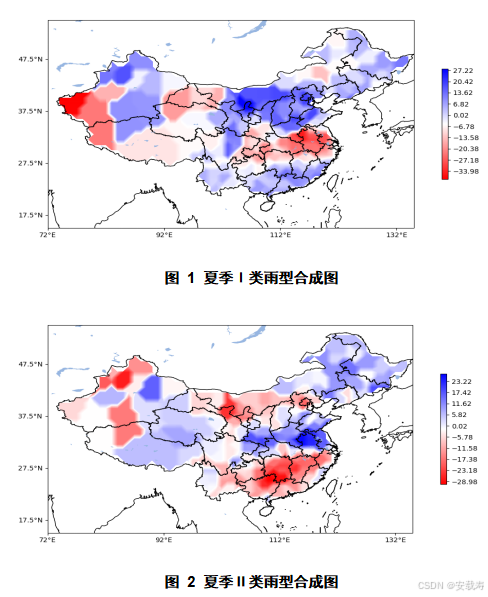
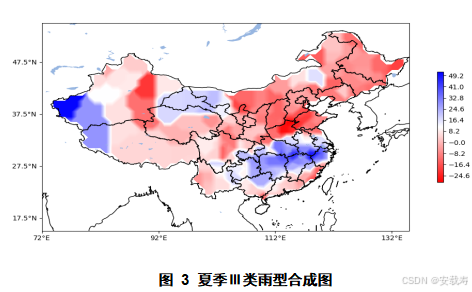
        图1至图3是1951年-2010年夏季三类雨型年合成图。图1是Ⅰ类雨型，即北方型，多雨带位于黄河流域及其以北区域，江淮流域大范围少雨，而在我国南方为次要多雨；图2是Ⅱ类雨型，多雨带位于黄河长江之间，雨带中心位于淮河流域，黄河以北，长江以南地区少雨；图三是Ⅲ类雨型，多雨带位于长江流域，淮河以北，我国东南沿海为少雨区。

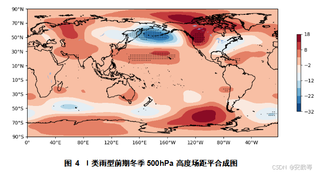
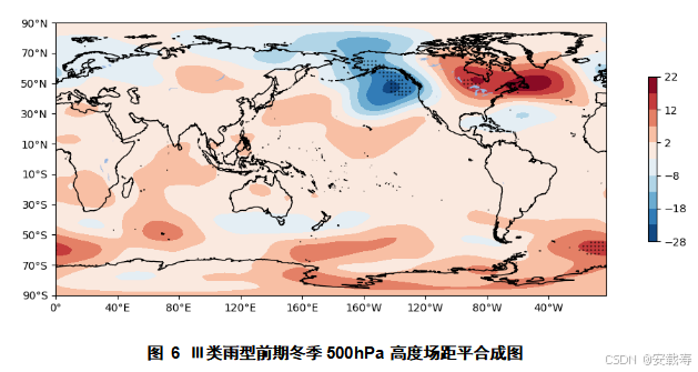
        图4至图6是各类雨型前期冬季500hPa高度场距平合成图。图4和图6中阿留申群岛和北美西部太平洋上空对应高度场偏低，而且该区域通过0.05显著性水平的总体均值t检验（点状阴影部分），说明该区域的高度场是显著不同于气候态，该区域高度场显著偏低，即位于阿留申地区的低压显著加深。同理在图4中北太平洋副热带地区和北美西部上空高度场显著增高，图6中北美中部上空高度场显著增高，图5中相反，阿留申群岛上空高度场显著增高，而北太平洋副热带地区和北美上空高度场显著偏低。从北太平洋和北美500hPa高度场高低压分布来看，可能是太平洋北美型遥相关（PNA），该遥相关型表现为热带和副热带太平洋高压加强，位于阿留申地区的低压加深，位于北美的脊加强，美国东部的槽加深。

        图4高度场分布对应着我国Ⅰ类雨型，可以看到，北太平洋副热带地区的高压显著加强，我国东南沿海地区可能受到副热带高压控制，降水较少，同时来自大洋水汽沿着副高边缘东南气流北上到达我国北方，同时在黄土高原的抬升作用下形成降雨，使得降水偏多。图5高度场分布与Ⅱ类雨型对应，副热带高压显著偏弱，远离我国东部，同时水汽无法深入到我国北方，北方降水减少，江淮流域降水偏多。图6高度场与Ⅲ类雨型对应，副热带高压偏强，但并不显著，同时强度低于图4中的副高，此时我国长江流域降水偏多，淮河以北以及东南沿海降水偏少。

 由于本人水平限制，多有错误，欢迎批评指正！