roc曲线和pr曲线

一、pr曲线

P-R曲线：P为precision查准率，R为recall查全率，以查准率为纵轴、查全率为横轴作图，所以P-R曲线是反映了“查准率”与“查全率”之间的关系

对于二分问题，可将样本划分为：真正例TP，假正例FP，真反例TN，假反例FN

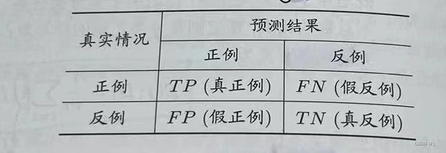
则查准率P=TP/(TP+FP)，查全率R=TP/(TP+FN)

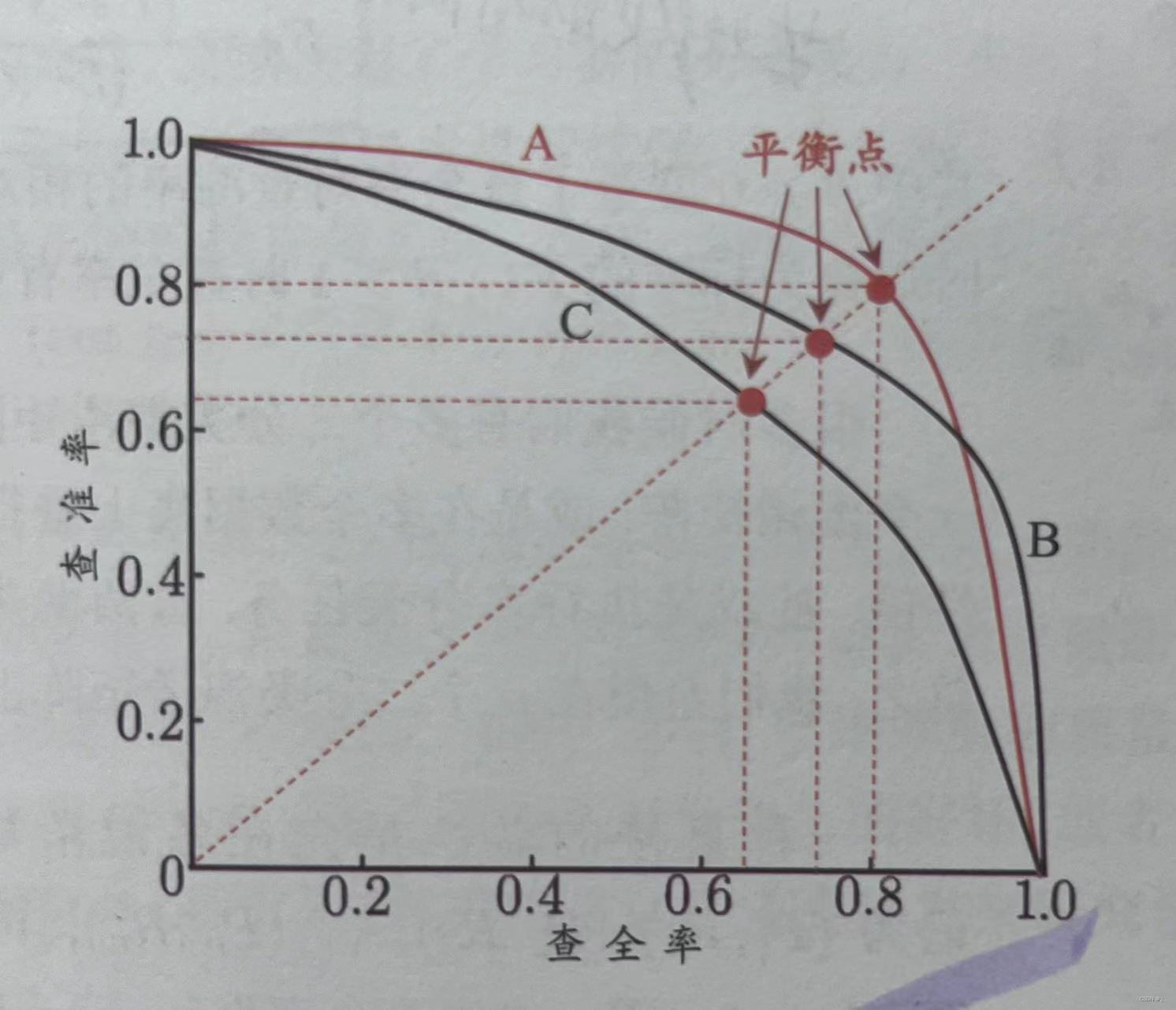
PR曲线越靠近右上角越好；平衡点(查准率=查全率)越高越好

优点：PR曲线的两个指标都聚焦于正例。类别不平衡问题中主要关心正例，所以在此情况下PR曲线被广泛认为优于ROC曲线。

缺点：缺少对负例的关注

二、roc曲线

ROC全称Receiver Operating Characteristic，即接收器操做特征曲线，坐标图式的分析工具。

ROC曲线以真正例率TPR=TP/(TP+FN)为纵坐标，假正例率FPR=FP/(FP+TN)为横坐标绘制。

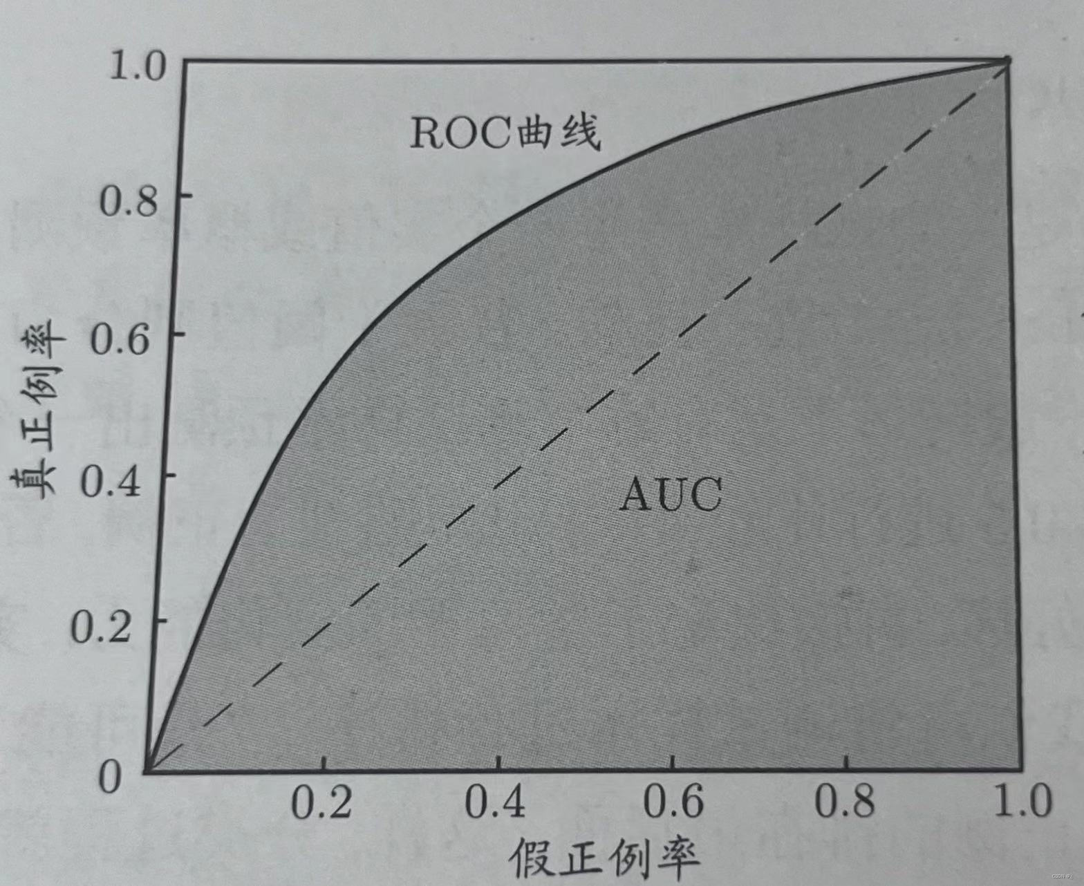
ROC曲线越靠近左上角，分类器的性能越好；如果越接近45度对角线，预测准确率越低。

若两条曲线发生交叉，曲线下面积AUC越大，预测准确率越高。

优点：1. 兼顾正例和负例的权衡。TPR聚焦于正例，FPR聚焦于与负例，是一个比较均衡的评估方法。2.TPR的分母是所有正例，FPR的分母是所有负例， 不依赖于具体的类别分布，不会随着类别分布的改变而改变

缺点：ROC曲线图上显示的不是真正的判断值；ROC曲线的绘图和用AUC进行分析比较繁琐。

三、曲线绘制

使用乳腺癌数据集，绘制PR曲线和ROC曲线。

#导入数据
import matplotlib.pyplot as plt
import numpy as np
from sklearn.datasets import load_breast_cancer
from sklearn.linear_model import LogisticRegression
#加载乳腺癌数据集
data = load_breast_cancer(as_frame=True)
X = data.data
y = data.target
#创建模型并训练
model = LogisticRegression()
model.fit(X, y)
#对样本进行预测，并计算预测得分
y_pred = model.predict(X)
scores = model.decision_function(X)
#计算准确率、召回率和阈值
def find_threshold(y_true, scores):
    fpr_list = []
    tpr_list = []
    precision_list = []
    recall_list = []
    thresholds = np.unique(scores)
    for threshold in thresholds:
        y_pred = np.zeros_like(y_true)
        y_pred[scores >= threshold] = 1
        tp = np.sum((y_true == 1) & (y_pred == 1))
        fp = np.sum((y_true == 0) & (y_pred == 1))
        fn = np.sum((y_true == 1) & (y_pred == 0))
        tn = np.sum((y_true == 0) & (y_pred == 0))
        fpr = fp / (fp + tn)
        tpr = tp / (tp + fn)
        precision = tp / (tp + fp)
        recall = tp / (tp + fn)
        fpr_list.append(fpr)
        tpr_list.append(tpr)
        precision_list.append(precision)
        recall_list.append(recall)
    return fpr_list, tpr_list, precision_list, recall_list, thresholds
 
 
fpr_list, tpr_list, precision_list, recall_list, thresholds = find_threshold(y, scores)

绘制PR曲线：

plt.plot(recall_list, precision_list)
plt.xlabel('Recall')
plt.ylabel('Precision')
plt.title('PR Curve')
plt.show()

绘制ROC曲线：

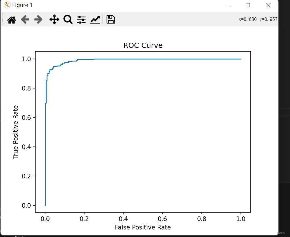
plt.plot(fpr_list, tpr_list)
plt.xlabel('False Positive Rate')
plt.ylabel('True Positive Rate')
plt.title('ROC Curve')
plt.show()

结果：