


超参数调整专题1
知识点回顾
1. 网格搜索
2. 随机搜索(简单介绍,非重点 实战中很少用到,可以不了解)
3. 贝叶斯优化(2种实现逻辑,以及如何避开必须用交叉验证的问题)
4. time库的计时模块,方便后人查看代码运行时长
今日作业:
对于信贷数据的其他模型,如LightGBM和KNN 尝试用下贝叶斯优化和网格搜索
步骤1:数据预处理
import pandas as pd
import pandas as pd    #用于数据处理和分析,可处理表格数据。
import numpy as np     #用于数值计算,提供了高效的数组操作。
import matplotlib.pyplot as plt    #用于绘制各种类型的图表
import seaborn as sns   #基于matplotlib的高级绘图库,能绘制更美观的统计图形。

 # 设置中文字体(解决中文显示问题)
plt.rcParams['font.sans-serif'] = ['SimHei']  # Windows系统常用黑体字体
plt.rcParams['axes.unicode_minus'] = False    # 正常显示负号
data = pd.read_csv('data.csv')    #读取数据

# 先筛选字符串变量
discrete_features = data.select_dtypes(include=['object']).columns.tolist()
# Home Ownership 标签编码
home_ownership_mapping = {
    'Own Home': 1,
    'Rent': 2,
    'Have Mortgage': 3,
    'Home Mortgage': 4
}
data['Home Ownership'] = data['Home Ownership'].map(home_ownership_mapping)

# Years in current job 标签编码
years_in_job_mapping = {
    '< 1 year': 1,
    '1 year': 2,
    '2 years': 3,
    '3 years': 4,
    '4 years': 5,
    '5 years': 6,
    '6 years': 7,
    '7 years': 8,
    '8 years': 9,
    '9 years': 10,
    '10+ years': 11
}
data['Years in current job'] = data['Years in current job'].map(years_in_job_mapping)

# Purpose 独热编码,记得需要将bool类型转换为数值
data = pd.get_dummies(data, columns=['Purpose'])
data2 = pd.read_csv("data.csv") # 重新读取数据,用来做列名对比
list_final = [] # 新建一个空列表,用于存放独热编码后新增的特征名
for i in data.columns:
    if i not in data2.columns:
       list_final.append(i) # 这里打印出来的就是独热编码后的特征名
for i in list_final:
    data[i] = data[i].astype(int) # 这里的i就是独热编码后的特征名


# Term 0 - 1 映射
term_mapping = {
    'Short Term': 0,
    'Long Term': 1
}
data['Term'] = data['Term'].map(term_mapping)
data.rename(columns={'Term': 'Long Term'}, inplace=True) # 重命名列
continuous_features = data.select_dtypes(include=['int64', 'float64']).columns.tolist()  #把筛选出来的列名转换成列表

 # 连续特征用中位数补全
for feature in continuous_features:
    mode_value = data[feature].mode()[0]            #获取该列的众数。
    data[feature].fillna(mode_value, inplace=True)          #用众数填充该列的缺失值,inplace=True表示直接在原数据上修改。
步骤二:划分数据
from sklearn.model_selection import train_test_split
X = data.drop(['Credit Default'], axis=1)  # 特征,axis=1表示按列删除
y = data['Credit Default'] # 标签
# 按照8:2划分训练集和测试集
X_train, X_test, y_train, y_test = train_test_split(X, y, test_size=0.2, random_state=42)  # 80%训练集,20%测试集
步骤三(一):网格搜索调参
3.1 网格搜索优化XGBoost
# --- 2. 网格搜索优化XGBoost ---
print("\n--- 2. 网格搜索优化XGBoost (训练集 -> 测试集) ---")
from xgboost import XGBClassifier
from sklearn.model_selection import GridSearchCV

# 定义XGBoost模型
xgb = XGBClassifier()

# 定义网格搜索参数
param_grid = {
    'n_estimators': [50, 100, 200],
    'max_depth': [None, 10, 20, 30],
    'min_child_weight': [1, 2, 4],
    'learning_rate': [0.01, 0.1, 0.2]
}

# 创建网格搜索对象
grid_search = GridSearchCV(estimator=xgb, param_grid=param_grid, cv=5, scoring='accuracy')

start_time = time.time()
# 在训练集上进行网格搜索
grid_search.fit(X_train, y_train)
end_time = time.time()

print(f"网格搜索耗时: {end_time - start_time:.4f} 秒")
print("最佳参数: ", grid_search.best_params_)

# 使用最佳参数的模型进行预测
best_model = grid_search.best_estimator_
best_pred = best_model.predict(X_test)

print("\n网格搜索优化后的XGBoost 在测试集上的分类报告:")
print(classification_report(y_test, best_pred))
print("网格搜索优化后的XGBoost 在测试集上的混淆矩阵:")
print(confusion_matrix(y_test, best_pred))
3.2 网格搜索优化 KNN
输入:
# --- 2. 网格搜索优化KNN ---
print("\n--- 2. 网格搜索优化KNN (训练集 -> 测试集) ---")
from sklearn.neighbors import KNeighborsClassifier
from sklearn.model_selection import GridSearchCV
# 定义KNN模型
knn = KNeighborsClassifier()
# 定义网格搜索参数
param_grid = {
'n_neighbors': [3, 5, 7, 9],
'weights': ['uniform', 'distance'],
'algorithm': ['auto', 'ball_tree', 'kd_tree', 'brute']
}
# 创建网格搜索对象
grid_search = GridSearchCV(estimator=knn, param_grid=param_grid, cv=5, scoring='accuracy')
start_time = time.time()
# 在训练集上进行网格搜索
grid_search.fit(X_train, y_train)
end_time = time.time()
print(f"网格搜索耗时: {end_time - start_time:.4f} 秒")
print("最佳参数: ", grid_search.best_params_)
# 使用最佳参数的模型进行预测
best_model = grid_search.best_estimator_
best_pred = best_model.predict(X_test)
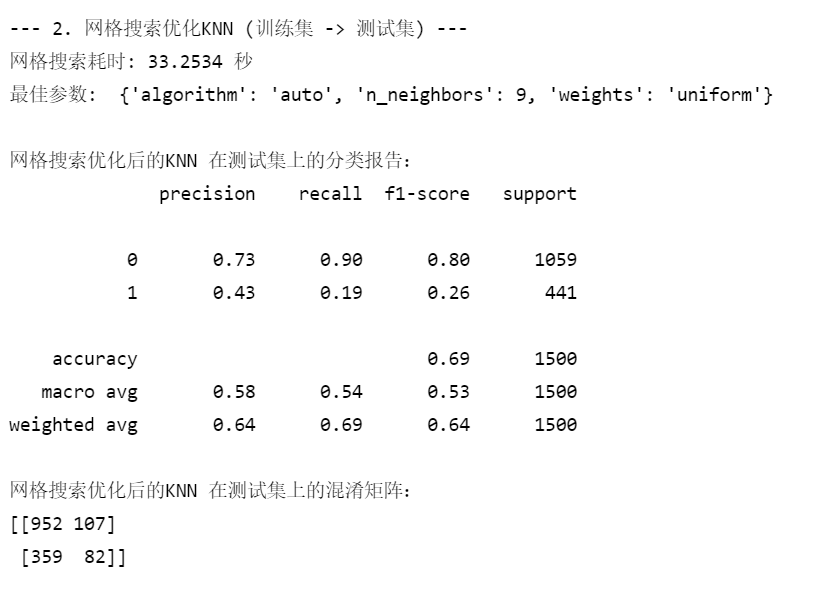
print("\n网格搜索优化后的KNN 在测试集上的分类报告:")
print(classification_report(y_test, best_pred))
print("网格搜索优化后的KNN 在测试集上的混淆矩阵:")
print(confusion_matrix(y_test, best_pred))输出:
3.3 网格搜索(Grid Search)超参数优化笔记
3.3.1、网格搜索基础概念
1. 核心思想
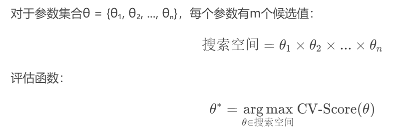
网格搜索是一种穷举搜索的超参数优化方法,通过:
-
预先定义参数的候选值范围
-
对所有可能的参数组合进行尝试
-
通过交叉验证评估每组参数的表现
-
最终选择性能最佳的参数组合
2. 数学表达
3.3.2 Scikit-learn实现详解
1 基本使用模板
from sklearn.model_selection import GridSearchCV
from sklearn.ensemble import RandomForestClassifier
# 定义参数网格
param_grid = {
'n_estimators': [50, 100, 200],
'max_depth': [3, 5, 7, None],
'min_samples_split': [2, 5, 10]
}
# 创建搜索器
grid_search = GridSearchCV(
estimator=RandomForestClassifier(random_state=42),
param_grid=param_grid,
cv=5, # 5折交叉验证
scoring='accuracy', # 评估指标
n_jobs=-1, # 使用所有CPU核心
verbose=1 # 显示进度
)
# 执行搜索
grid_search.fit(X_train, y_train)
# 输出结果
print("最佳参数:", grid_search.best_params_)
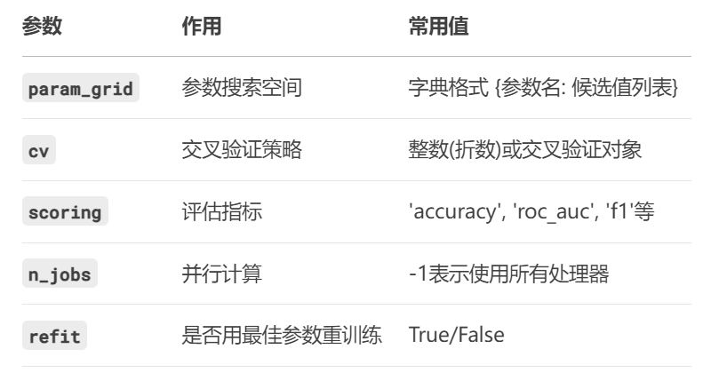
print("最佳分数:", grid_search.best_score_)2. 关键参数说明
步骤三(二):网格搜索调参
4.1 贝叶斯优化KNN
# --- 2. 贝叶斯优化XGBoost ---
print("\n--- 2. 贝叶斯优化XGBoost (训练集 -> 测试集) ---")
from skopt import BayesSearchCV
from skopt.space import Integer, Real
from xgboost import XGBClassifier
from sklearn.metrics import classification_report, confusion_matrix
import time

# 定义要搜索的参数空间
search_space = {
    'n_estimators': Integer(50, 200),
    'max_depth': Integer(10, 30),
    'learning_rate': Real(0.01, 0.2, prior='log-uniform'),
    'min_child_weight': Integer(1, 4)
}

# 创建贝叶斯优化搜索对象
bayes_search = BayesSearchCV(
    estimator=XGBClassifier(random_state=42),
    search_spaces=search_space,
    n_iter=32,  # 迭代次数,可根据需要调整
    cv=5, # 5折交叉验证,这个参数是必须的,不能设置为1,否则就是在训练集上做预测了
    n_jobs=-1,
    scoring='accuracy'
)

start_time = time.time()
# 在训练集上进行贝叶斯优化搜索
bayes_search.fit(X_train, y_train)
end_time = time.time()

print(f"贝叶斯优化耗时: {end_time - start_time:.4f} 秒")
print("最佳参数: ", bayes_search.best_params_)

# 使用最佳参数的模型进行预测
best_model = bayes_search.best_estimator_
best_pred = best_model.predict(X_test)

print("\n贝叶斯优化后的XGBoost 在测试集上的分类报告:")
print(classification_report(y_test, best_pred))
print("贝叶斯优化后的XGBoost 在测试集上的混淆矩阵:")
print(confusion_matrix(y_test, best_pred))
4.2 贝叶斯优化KNN
# ---  贝叶斯优化KNN ---
print("\n---  贝叶斯优化KNN (训练集 -> 测试集) ---")
from skopt import BayesSearchCV
from skopt.space import Integer, Categorical
from sklearn.neighbors import KNeighborsClassifier
from sklearn.metrics import classification_report, confusion_matrix
import time

# 定义要搜索的参数空间
search_space = {
    'n_neighbors': Integer(3, 15),
    'weights': Categorical(['uniform', 'distance']),
    'algorithm': Categorical(['auto', 'ball_tree', 'kd_tree', 'brute'])
}

# 创建贝叶斯优化搜索对象
bayes_search = BayesSearchCV(
    estimator=KNeighborsClassifier(),
    search_spaces=search_space,
    n_iter=32,  # 迭代次数,可根据需要调整
    cv=5, # 5折交叉验证
    n_jobs=-1,
    scoring='accuracy'
)

start_time = time.time()
# 在训练集上进行贝叶斯优化搜索
bayes_search.fit(X_train, y_train)
end_time = time.time()

print(f"贝叶斯优化耗时: {end_time - start_time:.4f} 秒")
print("最佳参数: ", bayes_search.best_params_)

# 使用最佳参数的模型进行预测
best_model = bayes_search.best_estimator_
best_pred = best_model.predict(X_test)

print("\n贝叶斯优化后的KNN 在测试集上的分类报告:")
print(classification_report(y_test, best_pred))
print("贝叶斯优化后的KNN 在测试集上的混淆矩阵:")
print(confusion_matrix(y_test, best_pred))
4.3 贝叶斯优化笔记
4.3.1 核心概念与原理
1. 基本思想
贝叶斯优化是一种序列化模型超参数优化方法,通过:
-
建立代理模型(通常是高斯过程)来近似目标函数
-
使用采集函数(Acquisition Function)决定下一个评估点
-
迭代更新代理模型,逐步逼近最优解
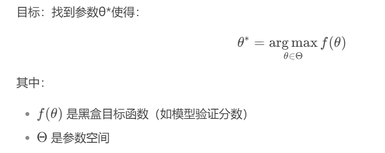
2. 数学框架
4.3.2 两种主流实现方式
方法1:基于scikit-optimize的实现
from skopt import BayesSearchCV
from skopt.space import Real, Integer, Categorical

# 定义搜索空间
search_spaces = {
    'learning_rate': Real(0.01, 0.2, prior='log-uniform'),
    'max_depth': Integer(3, 7),
    'subsample': Real(0.6, 1.0),
    'colsample_bytree': Real(0.6, 1.0)
}

# 创建贝叶斯优化器
opt = BayesSearchCV(
    estimator=XGBClassifier(random_state=42),
    search_spaces=search_spaces,
    n_iter=32,                   # 迭代次数
    cv=5,                        # 交叉验证折数
    scoring='roc_auc',
    n_jobs=-1,
    random_state=42
)

# 执行优化
opt.fit(X_train, y_train)

# 输出结果
print("最佳参数:", opt.best_params_)
print("最佳分数:", opt.best_score_)
方法2:基于Optuna的实现(更灵活)
import optuna
from sklearn.metrics import log_loss

def objective(trial):
    params = {
        'learning_rate': trial.suggest_float('learning_rate', 0.01, 0.2, log=True),
        'max_depth': trial.suggest_int('max_depth', 3, 7),
        'subsample': trial.suggest_float('subsample', 0.6, 1.0),
        'colsample_bytree': trial.suggest_float('colsample_bytree', 0.6, 1.0)
    }

    # 单次训练-验证拆分(避免交叉验证开销)
    X_tr, X_val, y_tr, y_val = train_test_split(X_train, y_train, test_size=0.2)

    model = XGBClassifier(**params, random_state=42)
    model.fit(X_tr, y_tr)

    y_pred = model.predict_proba(X_val)
    return log_loss(y_val, y_pred)  # 最小化目标

# 创建并运行研究
study = optuna.create_study(direction='minimize')
study.optimize(objective, n_trials=50)

# 结果分析
print("最佳参数:", study.best_params)
print("最佳分数:", study.best_value)
4.3.3 关键组件详解
1. 参数空间定义
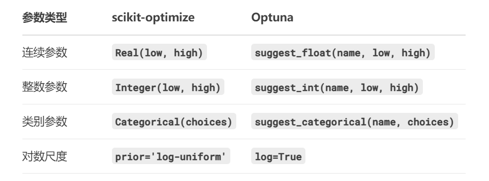
2. 采集函数(Acquisition Function)
常用类型:
-
EI (Expected Improvement):期望提升
-
PI (Probability of Improvement):提升概率
-
UCB (Upper Confidence Bound):上置信界
Optuna默认使用TPE(Tree-structured Parzen Estimator),适合混合类型参数
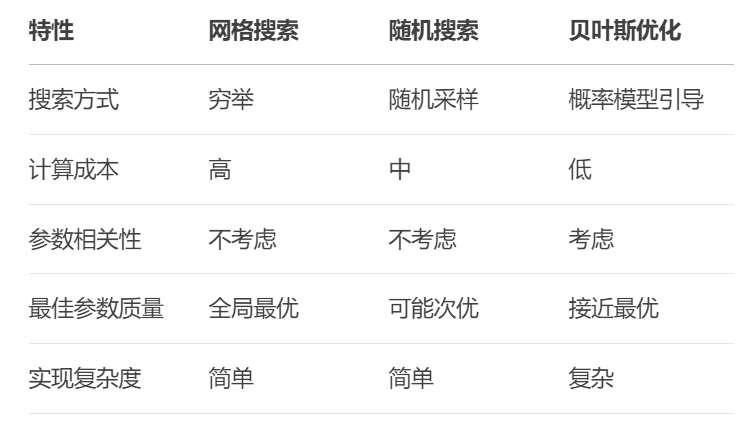
4.4 本节课三种算法比较


 185
185

 被折叠的 条评论
为什么被折叠?
被折叠的 条评论
为什么被折叠?
 到【灌水乐园】发言


