销售分析项目

 项目需求
- 对一家日用品销售数据进行 “人、货、场”分析，并给出提升销量的针对性建议。
    - 人：对客户进行价值分析。分析客户类型与销售贡献比、基于RFM模型的用户行为分析。
    - 货：商品分析。了解在售商品结构（品类，价格带，折扣带）找出优势/爆款商品、劣势/待优化商品。
    - 场：对统计周期内的运营情况进行分析。
         - 市场布局分析：对全球不同分店盈利情况进行分析，各国盈利情况进行分析。
         - 促销活动分析
         - 盈利情况分析：根据一些盈利指标（销售额、利润额、利润率、销售量）对盈利情况进行分析；时间维度分析，发现规律。

- 数据集介绍
    - Row_ID：行编号
    - Order_ID：订单ID
    - Order_Date：订单日期
    - Ship_Date：发货时间
    - Ship_Mode：发货模式
    
    - Customer_ID：客户ID
    - Customer_Name：客户姓名
    - Segment：客户类别
    - City：客户所在城市
    - State：客户城市所在州
    - Country：客户所在国家
    
    - Postal_Code：邮编   
    - Market：分店所属区域
    - Region：分店所属州
    - Product_ID：产品ID
    - Category：商品类别
    - Sub_Category：产品子类别
    - Product_Name：产品名称
    
    - Sales：销售额
    - Quantity：销售量
    - Discount：折扣
    - Profit：利润
    - Shipping Cost：发货成本
    - Order_Priority：订单优先级

1.数据加载和预览

import pandas as pd
import numpy as np
import matplotlib.pyplot as plt
import warnings
plt.rcParams['font.sans-serif'] = ['Microsoft YaHei']
plt.rcParams['axes.unicode_minus'] = False 
warnings.filterwarnings('ignore')
# 导入数据
df = pd.read_csv('sale_data.csv',encoding='ISO-8859-1')
df.head(2)

df.shape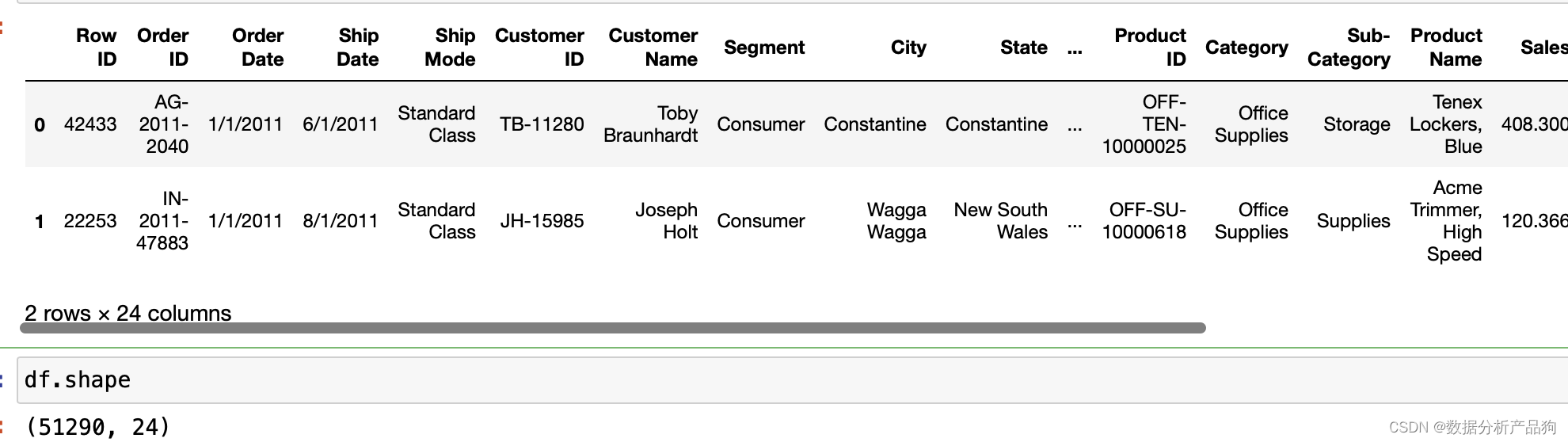

数据格式很多不对的，考虑进行格式修正及清洗。

2.数据处理

df.columns #查看所有的列索引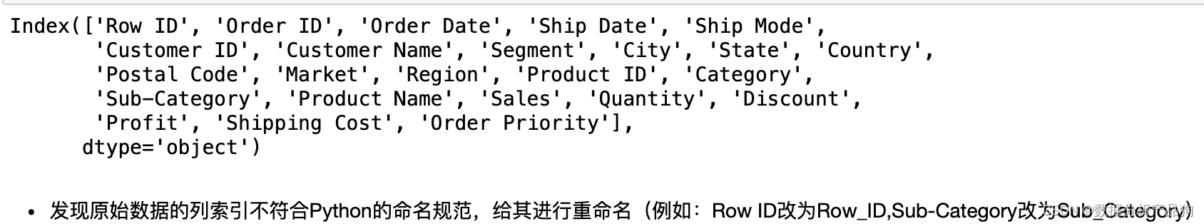

#修改列索引
df.rename(columns= lambda x:x.replace(' ','_').replace('-','_'),inplace= True)
df.columns 
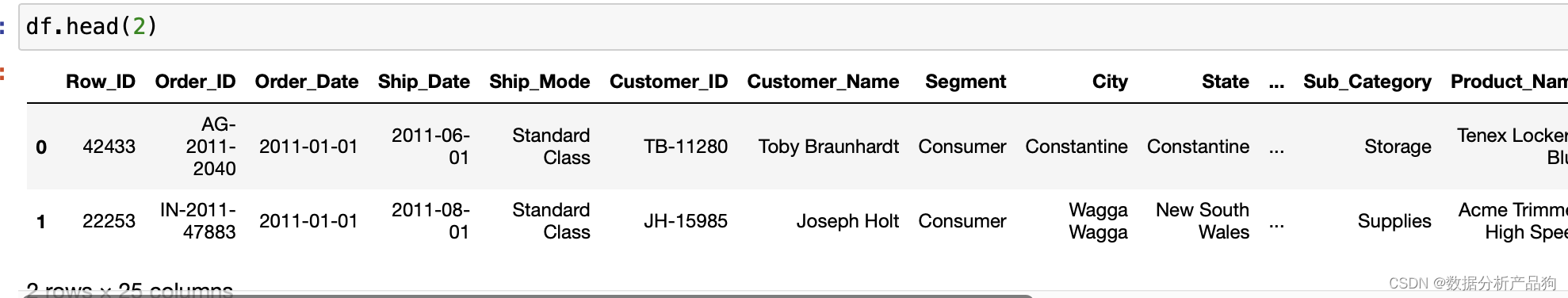
#修改时间类型
df['Order_Date'] = pd.to_datetime(df['Order_Date'])
df['Ship_Date'] = pd.to_datetime(df['Ship_Date'])

# 为了方便分析每年和每月的销售情况，把年份和月份提取出
df['year'] = df['Order_Date'].dt.year  #添加一列‘年份’（.dt.year）
df['month'] = df['Order_Date'].values.astype('datetime64[M]')
 #添加一列‘month’取出列，修改类型，提取带年份的月

#空置识别
df.isnull().any(axis=0) #发现Postal_Code 列存在空值
#查看空值占比情况
df['Postal_Code'].isnull().sum()/df['Row_ID'].size
#空值占比较大可以考虑删除
df.drop(columns='Postal_Code',inplace=True)

#查看重复数据
df.duplicated().sum() 

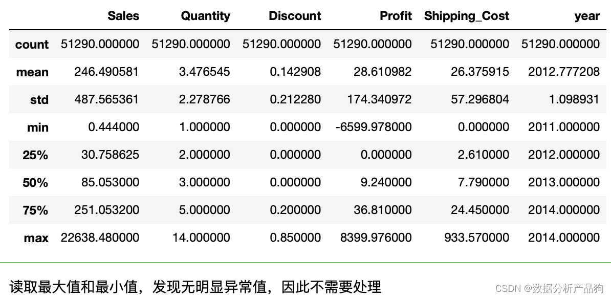
#检测异常值
df['Row_ID']=df['Row_ID'].astype('str')#转为字符串类型
df.describe() #只对时间和数字类型做统计描述

3.数据分析

3.1 用户分析

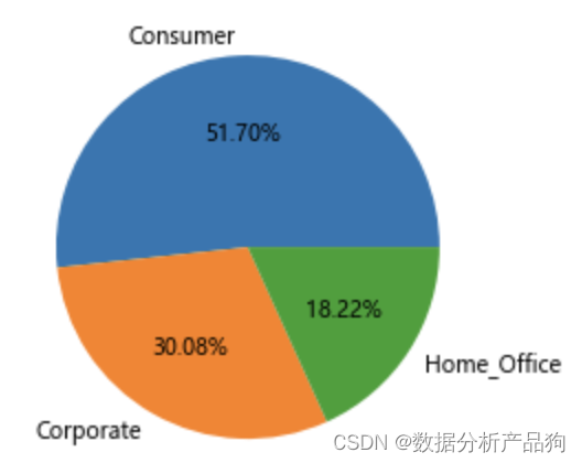
不同类别客户分析

segment_year = df.groupby(by=['Segment','year'])['Customer_ID'].nunique().reset_index()
segment_year

#查看每年不同类型客户数量情况
import seaborn as sns #sns可以绘制分组柱状图
sns.barplot(x='Segment',y='Customer_ID',hue='year',data=segment_year)

查看每年用户增长情况

# 查看不同类型客户每年贡献的销售额
segment_sales = df.groupby(by=['Segment','year'])['Sales'].sum().reset_index()
sns.barplot(x='Segment',y='Sales',hue='year',data=segment_sales)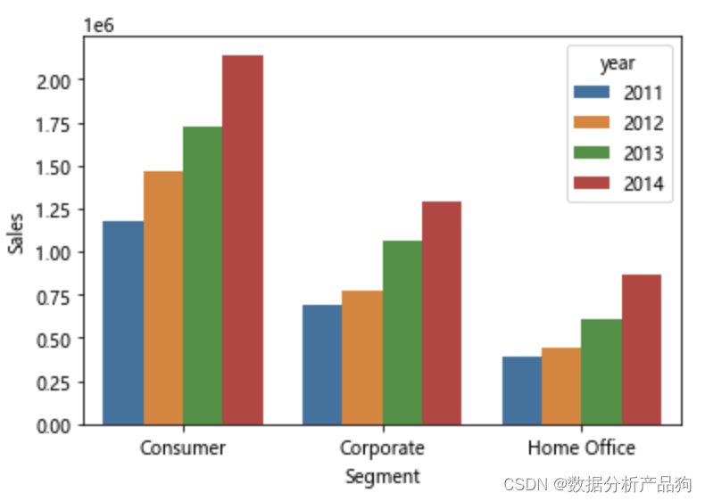

可以看出，各个类型的客户每年贡献的销售额都在稳步提升，普通消费者贡献的销售额最多，这和客户占比也有一定关系，因为普通用户占比最多。

3.1.1客户下单行为分析

#首先截取Customer_ID, Order_Date为新的子集，叫做”下单客户集“，并对Order_Date进行排序，方便后续分析 
customer_buy_df = df[['Customer_ID','Order_Date']].sort_values(['Order_Date'])
customer_buy_df.head(3)

#查看所有用户第一次购买的日期分布和人数统计
customer_buy_df.groupby(by='Customer_ID')['Order_Date'].min().value_counts().plot()

#查看所有用户最后一次购买的日期分布和人数统计
customer_buy_df.groupby(by='Customer_ID')['Order_Date'].max().value_counts().plot()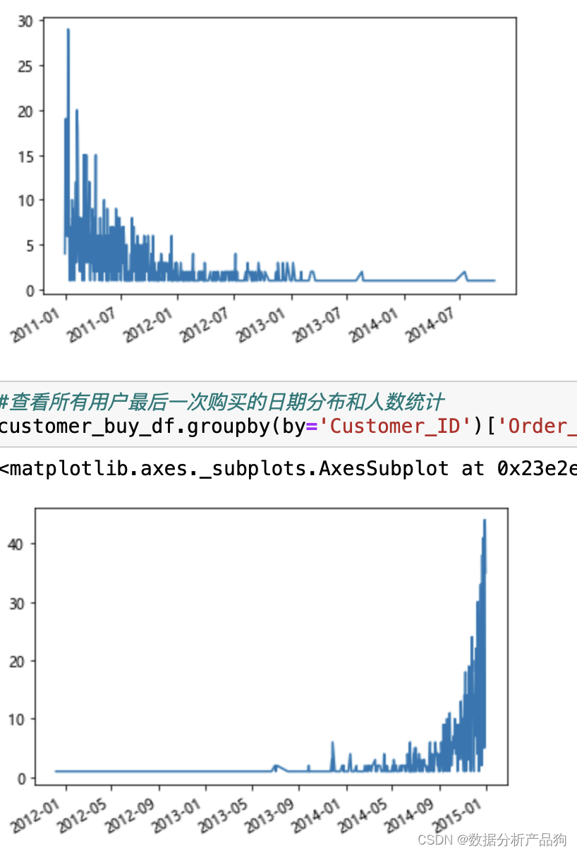

可以看出， 在所有用户第一次购买的日期分布和人数统计统计图表中，13年初以后新用户增长的趋势缓慢，商家可以通过广告等推广策略吸收更多的新用户；
而通过观察所有用户最后一次购买的日期分布和人数统计的图表，可以发现用户基本没有流失（12-14年间，15年1月份看上去用户流失多，是因为用户可能会在15年2月份继续消费，而本数据的统计时间结点为15年1月份），也验证了每年销售额的增长趋势。

#查看新老用户的占比
customer_df = customer_buy_df.groupby(by='Customer_ID')['Order_Date'].agg(['max','min'])
(customer_df['min'] == customer_df['max']).value_counts()

False    1580
True       10
dtype: int64 #只有10个新用户，可见老用户比较多

3.1.2 RFM模型分析

- R（Recency）：客户最近一次交易时间的间隔。R值越大，表示客户交易发生的日期越久，反之则表示客户交易发生的日期越近。
- F（Frequency）：客户在最近一段时间内交易的次数。F值越大，表示客户交易越频繁，反之则表示客户交易不够活跃。
- M（Monetary）：客户在最近一段时间内交易的金额。M值越大，表示客户价值越高，反之则表示客户价值越低。

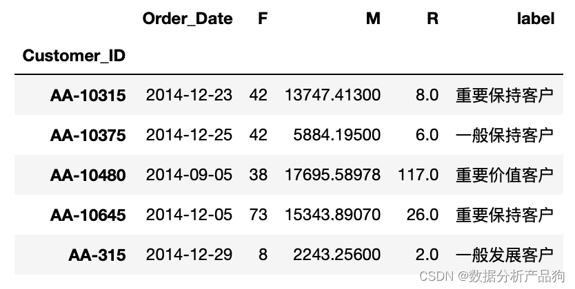
#构建RFM表
#基于Customer_ID分类，依次求出每个下单客户的总消费金额，最后一次消费时间和总消费次数（总订单量）
rfm = df.pivot_table(index='Customer_ID',values=['Order_ID','Sales','Order_Date'],aggfunc={'Order_ID':'count','Sales':'sum','Order_Date':'max'})
rfm['R'] = (rfm['Order_Date'].max() - rfm['Order_Date'])/np.timedelta64(1,'D')
rfm.rename(columns={'Order_ID':'F','Sales':'M'},inplace=True)
rfm.head()

#计算R，F和M列中元素距均值的距离
distance = rfm[['R','F','M']].apply(lambda x:x-x.mean(),axis=0)

#进行价值分层
def rfm_func(x):
    level = x.map(lambda y:'1' if y > 0 else '0')
    level = level['R'] + level['F'] + level['M']
    d = {
        '111':'重要价值客户',
        '011':'重要保持客户',
        '101':'重要挽留客户',
        '001':'重要发展客户',
        '110':'一般价值客户',
        '010':'一般保持客户',
        '100':'一般挽留客户',
        '000':'一般发展客户'
    }
    result = d[level]
    return result
rfm['label'] = distance.apply(rfm_func,axis=1)
rfm.head()

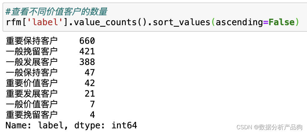
3.2商品情况分析

找到销量、销售额、利润Top10的商品

#销量Top10
product_count_top_10 = df.groupby(by='Product_ID')['Customer_ID'].count().sort_values(ascending=False)[:10]
product_count_top_10
#销售额top10
product_amount_top_10 = df.groupby(by='Product_ID')['Sales'].sum().sort_values(ascending=False)[:10]
product_amount_top_10
#利润top10的商品
product_profit_top_10 = df.groupby(by='Product_ID')['Profit'].sum().sort_values(ascending=False)[:10]
product_profit_top_10

查看商品种类的销售情况

#将商品的大类和小类数据组合到一起，形成df中新的一列商品的详细类别：Category_Sub_Category
df['Category_Sub_Category'] = df[['Category','Sub_Category']].apply(lambda x:x[0]+'_'+x[1],axis=1)
df.head()

#计算计算不同详细类别商品的总利润和总销售额,然后根据销售额进行降序
df_Category_Sub_Category = df.groupby(by='Category_Sub_Category').agg({'Profit':'sum','Sales':'sum'}).reset_index().sort_values(by='Sales',ascending=False)
df_Category_Sub_Category

发现个别利润为负的产品，那就是这个商品在亏损情况。

#检查桌子Tables的原始数据，查看是否存在打折？
tables_df = df.loc[df['Sub_Category'] == 'Tables']
tables_s = tables_df['Discount'].value_counts()

#计算打折率 打折的桌子数/总桌子数
discount_rate = tables_s.iloc[1:].sum() / tables_s.sum()
discount_rate

Bookcases_df = df.loc[df['Sub_Category'] == 'Bookcases']
Bookcases_s = Bookcases_df['Discount'].value_counts()
discount_rate = Bookcases_s.iloc[1:].sum() / Bookcases_s.sum()
discount_rate

通过检查原数据，发现Ta大部分都在打折，打折的销量高达75.8%。Boo打折销量高达0.53% 如果是在清库存，这个效果还是不错的. 但如果不是，说明这个产品在市场推广上遇到了瓶颈需要适当改善经营策略。

3.3整体销售情况分析

首先构造整体销售情况子数据集，销售情况主要需要观察如下字段，包含：订单日期、销售额、销售量、利润、年份和月份。

sales_data = df[['Order_Date','Sales','Quantity','Profit','year','month']]
sales_data.head()
sales_year = sales_data.groupby(by=['year','month']).sum()
sales_year
#为了方便观察将不同年份的数据以单表进行存储显示，构建的时候重新设置行索引
year_2011 = sales_year.loc[2011].reset_index()
year_2012 = sales_year.loc[2012].reset_index()
year_2013 = sales_year.loc[2013].reset_index()
year_2014 = sales_year.loc[2014].reset_index()

3.4销售额分析

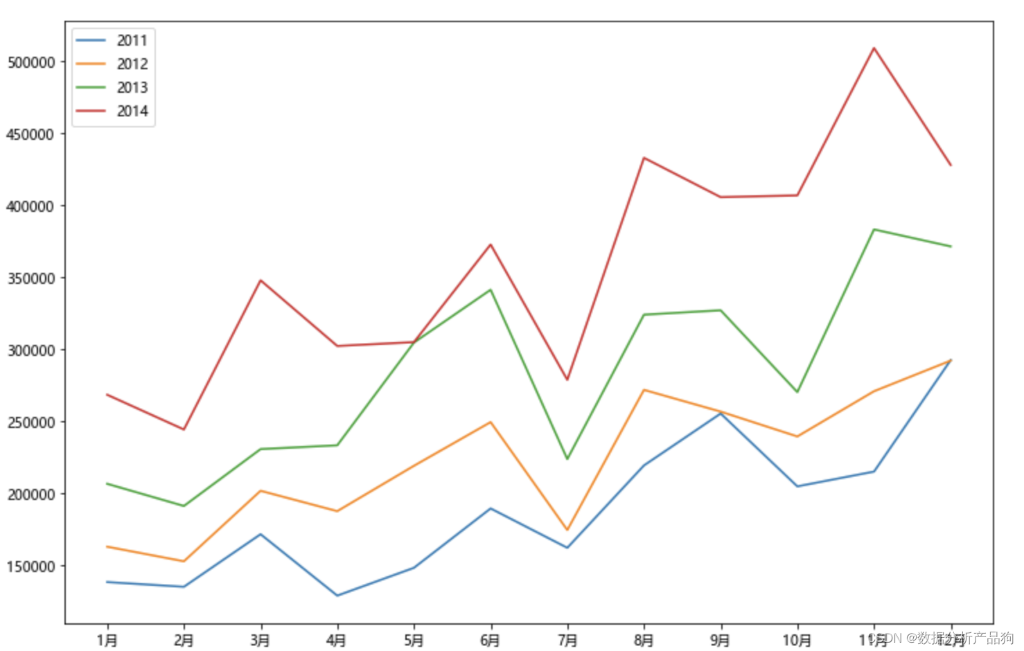
sales = pd.concat([year_2011['Sales'],year_2012['Sales'],year_2013['Sales'],year_2014['Sales']],axis=1)###水平级联
#对行和列进行重命名
sales.columns = ['Sales_2011','Sales_2012','Sales_2013','Sales_2014']
sales.index = ['1月','2月','3月','4月','5月','6月','7月','8月','9月','10月','11月','12月']

#设置表格背景色显示，销售额越高，则颜色越深
sales.style.background_gradient(axis=0) #以列为单位

可以看到，下半年整体销售情况比上半年好一些，同时，随着年份的增大，销售额也有明显的增加，说明销售业绩增长较快，整体发展呈现良性循环。

3.4.1分析年销售总额和增长率

从上面表格显示增长率的结果可知，后两年的销售总额的增长率达到了26%以上，14年的增长率几乎达到了12年的两倍，发展势头良好，经营在稳定增长。

3.5不同年份的销量取出，构建销量表

quantity = pd.concat([year_2011['Quantity'],year_2012['Quantity'],year_2013['Quantity'],year_2014['Quantity']],axis=1)
#对行和列进行重命名
quantity.columns = ['Quantity_2011','Quantity_2012','Quantity_2013','Quantity_2014']
quantity.index = ['1月','2月','3月','4月','5月','6月','7月','8月','9月','10月','11月','12月']

#设置表格显示，销售额越高，则颜色越深
quantity.style.background_gradient(axis=0) 

 

#计算增长率:后一年的总销量 / 前一年的总销量 - 1
rise_rate = (quantity_sum[1:].values / quantity_sum[0:-1].values) - 1
rise_rate = rise_rate.tolist()
rise_rate.insert(0,0) #补充无法计算的第一年的增长率

#汇总到df表格中进行显示
quantity_df = pd.DataFrame({'quantity_sum':quantity_sum,'rise_rate':rise_rate})
quantity_df['rise_rate'] = quantity_df['rise_rate'].map(lambda x:format(x,'.2%'))
quantity_df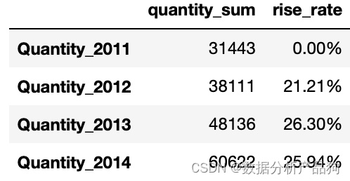

#利润分析
profit = pd.concat([year_2011['Profit'],year_2012['Profit'],year_2013['Profit'],year_2014['Profit']],axis=1)
#对行和列进行重命名
profit.columns = ['Profit-2011','Profit-2012','Profit-2013','Profit-2014']
profit.index = ['1月','2月','3月','4月','5月','6月','7月','8月','9月','10月','11月','12月']
#设置表格显示，销售额越高，则颜色越深
profit.style.background_gradient(axis=0) 

#计算每年度利润总额并画图显示
profit_sum = profit.sum(axis=0)
plt.bar(profit_sum.index,profit_sum.values)

#计算利润率
profit_rate = profit_sum.values / sales_sum.values
profit_rate_df = pd.DataFrame(data=profit_rate,columns=['利润率'],index=['2011年','2012年','2013年','2014年'])
profit_rate_df['利润率'] = profit_rate_df['利润率'].map(lambda x:format(x,'.2%'))
profit_rate_df

建议，销售分布用Tableau等BI工具展示更为明显。