Deep learning 六

四、卷积神经网络的可视化

        卷积神经网络表示非常适合可视化，很大程度上是因为它们是视觉概念的表示。下面是三种最容易理解也最有用的方法

        可视化卷积神经网络的中间输出(中间激活):有助于理解卷积神经网络连续的层如何对输人进行变换，也有助于初步了解卷积神经网络每个过滤器的含义。

        可视化卷积神经网络的过滤器:有助于精确理解卷积神经网络中每个过滤器容易接受的
视觉模式或视觉概念
        可视化图像中类激活的热力图:有助于理解图像的哪个部分被识别为属于某个类别，从而可以定位图像中的物体。

1.可视化中间激活

        可视化中间激活，是指对于给定输入，展示网络中各个卷积层和池化层输出的特征图(层的输出通常被称为该层的激活，即激活函数的输出)。这让我们可以看到输入如何被分解为网络学到的不同过滤器。我们希望在三个维度对特征图进行可视化: 宽度、高度和深度(通道)。每个通道都对应相对独立的特征，所以将这些特征图可视化的正确方法是将每个通道的内容分别绘制成二维图像。我们首先来5.2节保存的模型。

from keras.models import load_model

model = load_model('cats_and_dogs_small_2.h5')
model.summary()  # As a reminder.

_________________________________________________________________
Layer (type)                 Output Shape              Param #   
=================================================================
conv2d_5 (Conv2D)            (None, 148, 148, 32)      896       
_________________________________________________________________
max_pooling2d_5 (MaxPooling2 (None, 74, 74, 32)        0         
_________________________________________________________________
conv2d_6 (Conv2D)            (None, 72, 72, 64)        18496     
_________________________________________________________________
max_pooling2d_6 (MaxPooling2 (None, 36, 36, 64)        0         
_________________________________________________________________
conv2d_7 (Conv2D)            (None, 34, 34, 128)       73856     
_________________________________________________________________
max_pooling2d_7 (MaxPooling2 (None, 17, 17, 128)       0         
_________________________________________________________________
conv2d_8 (Conv2D)            (None, 15, 15, 128)       147584    
_________________________________________________________________
max_pooling2d_8 (MaxPooling2 (None, 7, 7, 128)         0         
_________________________________________________________________
flatten_2 (Flatten)          (None, 6272)              0         
_________________________________________________________________
dropout_1 (Dropout)          (None, 6272)              0         
_________________________________________________________________
dense_3 (Dense)              (None, 512)               3211776   
_________________________________________________________________
dense_4 (Dense)              (None, 1)                 513       
=================================================================
Total params: 3,453,121
Trainable params: 3,453,121
Non-trainable params: 0
_________________________________________________________________

接下来，输入一张猫的图像，但它不属于网络的训练图像

"""预处理单张图像"""

img_path = '/Users/fchollet/Downloads/cats_and_dogs_small/test/cats/cat.1700.jpg'

# We preprocess the image into a 4D tensor
"""将图像预处理为一个4D张量"""
from keras.preprocessing import image
import numpy as np

img = image.load_img(img_path, target_size=(150, 150))
img_tensor = image.img_to_array(img)
img_tensor = np.expand_dims(img_tensor, axis=0)
# Remember that the model was trained on inputs
# that were preprocessed in the following way:
"""训练模型的输入数据都用这种方法预处理"""
img_tensor /= 255.

# Its shape is (1, 150, 150, 3)
print(img_tensor.shape)


"""显示测试图像"""
import matplotlib.pyplot as plt

plt.imshow(img_tensor[0])
plt.show()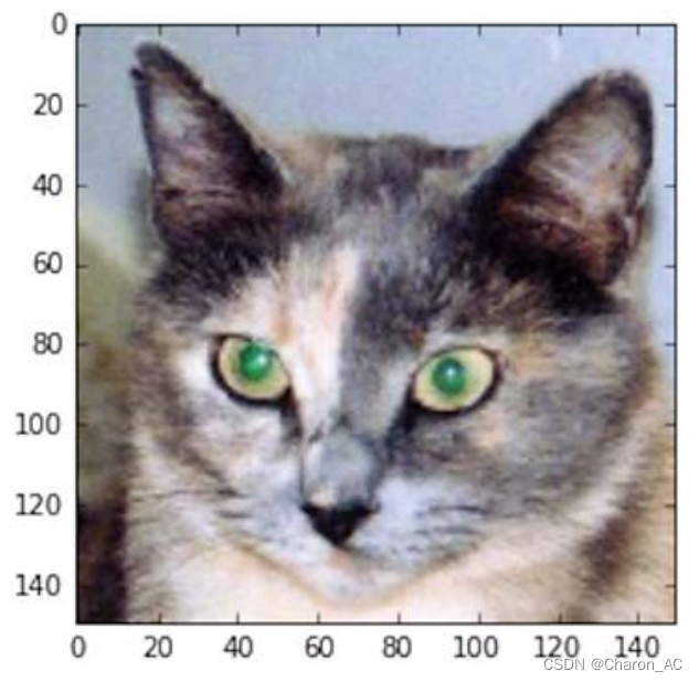

 为了提取想要查看的特征图，我们需要创建一个 Keras 模型，以图像批量作为输人，并输出所有卷积层和池化层的激活。为此，我们需要使用 Keras 的 Mode 类。模型实例化需要两个参数:一个输人张量(或输人张量的列表)和一个输出张量(或输出张量的列表)。得到的类是一个Keras模型，就像你熟悉的 sequential模型一样，将特定输人映射为特定输出。Model类允许模型有多个输出，这一点与 Sequential模型不同。

"""用一个输入张量和一个输出张量列表将模型实例化"""

from keras import models

# Extracts the outputs of the top 8 layers:
"""提取前8层的输出"""
layer_outputs = [layer.output for layer in model.layers[:8]]
# Creates a model that will return these outputs, given the model input:
"""创建一个模型，给定模型输入，可以返回这些输出"""
activation_model = models.Model(inputs=model.input, outputs=layer_outputs)


"""输入一张图像，这个模型将返回原始模型前8层的激活值，这个模型有一个输入和8个输出，每层激活对应一个输出"""


"""以预测模式运行模型"""
# This will return a list of 5 Numpy arrays:
# one array per layer activation
"""返回8个numpy数组组成的列表，每个层激活对应一个numpy数组"""
activations = activation_model.predict(img_tensor)

"""第一个卷积层的激活如下"""
first_layer_activation = activations[0]
print(first_layer_activation.shape)
(1, 148, 148, 32)

"""这是大小为148*148的特征图，有32个通道，来绘制原始模型第一层激活的第四个通道"""

"""将第四个通道可视化"""
import matplotlib.pyplot as plt

plt.matshow(first_layer_activation[0, :, :, 3], cmap='viridis')
plt.show()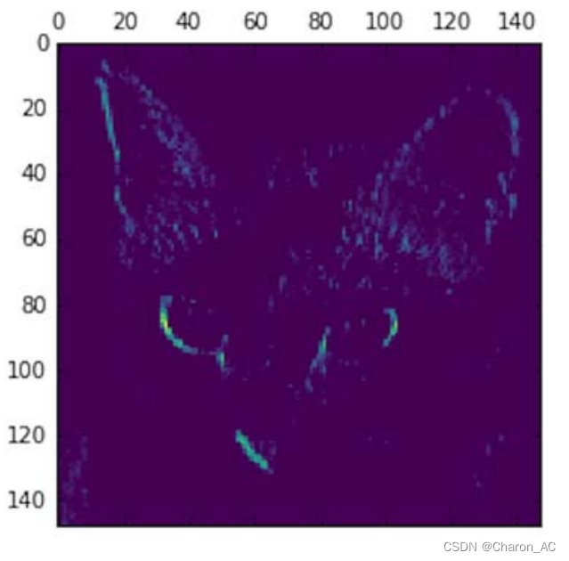

这个通道似乎是对角边缘检测器，再看一下第七个通道（运行出来可能不同，因为卷积层学到的过滤器并不是确定的）

"""将第七个通道可视化"""

plt.matshow(first_layer_activation[0, :, :, 30], cmap='viridis')
plt.show()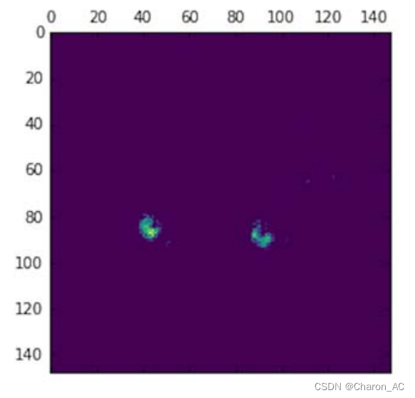

 

这个通道看起来像是“鲜绿色圆点”检测器，对寻找猫眼睛很有用。下面我们来绘制网络中所有激活的完整可视化。我们需要在8个特征图中的每一个中提取并绘制每一个通道，然后将结果叠加在一个大的图像张量中，按通道并排。 

"""将每个中间激活的所有通道可视化"""

import keras

# These are the names of the layers, so can have them as part of our plot
"""层的名称"""
layer_names = []
for layer in model.layers[:8]:
    layer_names.append(layer.name)

images_per_row = 16

# Now let's display our feature maps
"""显示特征图"""
for layer_name, layer_activation in zip(layer_names, activations):
    # This is the number of features in the feature map
    """特征图中的特征个数"""
    n_features = layer_activation.shape[-1]

    # The feature map has shape (1, size, size, n_features)
    """特征图的形状为（1，size, size, n_features）"""
    size = layer_activation.shape[1]

    # We will tile the activation channels in this matrix
    """在这个矩阵中将激活通道平铺"""
    n_cols = n_features // images_per_row
    display_grid = np.zeros((size * n_cols, images_per_row * size))

    # We'll tile each filter into this big horizontal grid
    """将每个过滤器平铺到一个大的水平网格中"""
    for col in range(n_cols):
        for row in range(images_per_row):
            channel_image = layer_activation[0,
                                             :, :,
                                             col * images_per_row + row]
            # Post-process the feature to make it visually palatable
            """对特征进行后处理，使其看起来更美观"""
            channel_image -= channel_image.mean()
            channel_image /= channel_image.std()
            channel_image *= 64
            channel_image += 128
            channel_image = np.clip(channel_image, 0, 255).astype('uint8')
            display_grid[col * size : (col + 1) * size, """显示网格"""
                         row * size : (row + 1) * size] = channel_image

    scale = 1. / size
    plt.figure(figsize=(scale * display_grid.shape[1],
                        scale * display_grid.shape[0]))
    plt.title(layer_name)
    plt.grid(False)
    plt.imshow(display_grid, aspect='auto', cmap='viridis')
    
plt.show()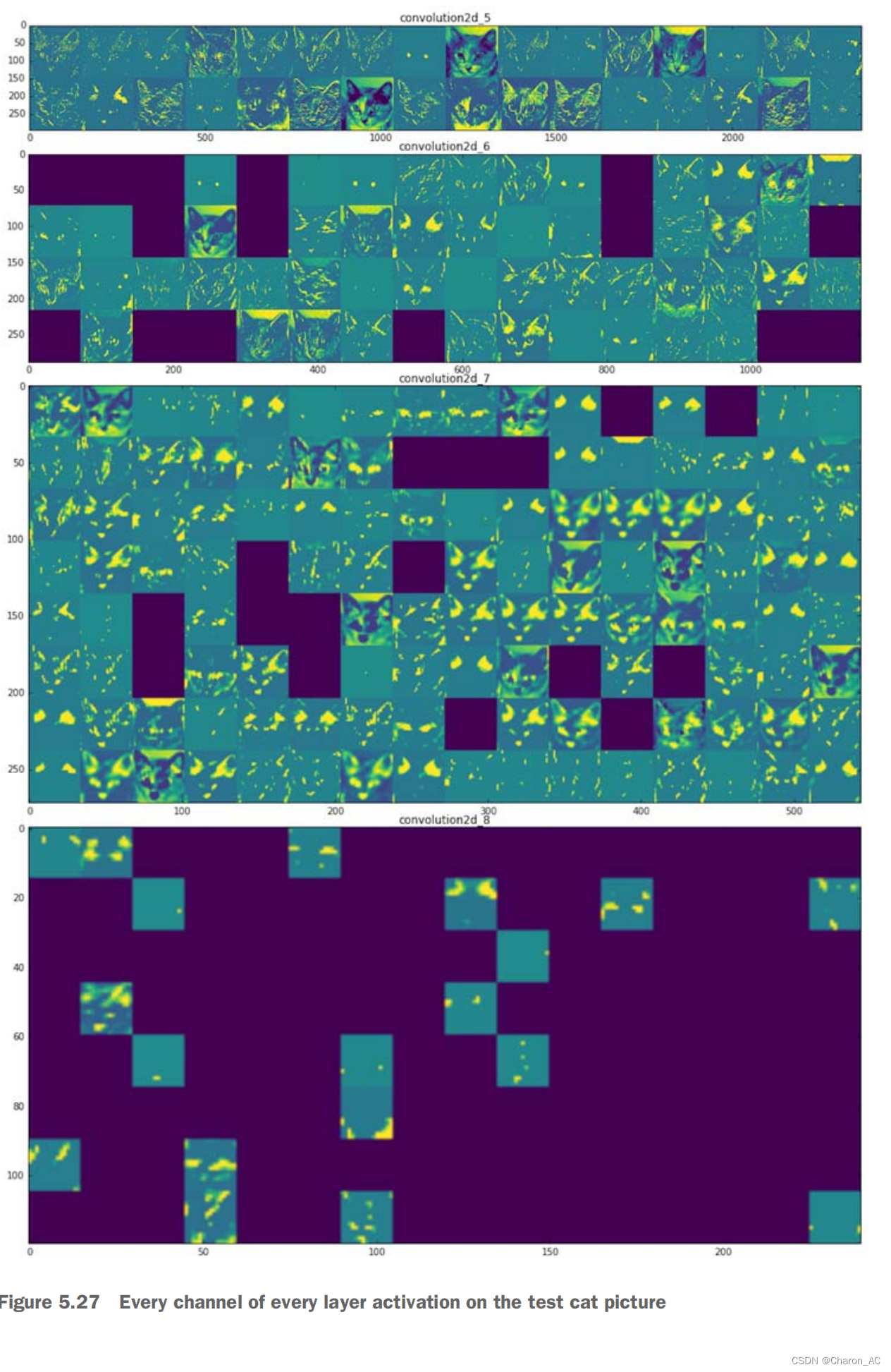

对于测试的猫图像，每个层激活的所有通道

这里需要注意以下几点。
        第一层是各种边缘探测器的集合。在这一阶段，激活几乎保留了原始图像中的所有信息。

        随着层数的加深，激活变得越来越抽象，并且越来越难以直观地理解。它们开始表示更高层次的概念，比如“猫耳朵”和“猫眼睛”。层数越深，其表示中关于图像视觉内容的信息就越少，而关于类别的信息就越多。
        激活的稀疏度(sparsity)随着层数的加深而增大。在第一层里，所有过滤器都被输入图像激活，但在后面的层里，越来越多的过滤器是空白的。也就是说，输人图像中找不到这些过滤器所编码的模式。 

这揭示了深度神经网络学到的表示的一个重要普遍特征:随着层数的加深，层所提取的特征变得越来越抽象。更高的层激活包含关于特定输入的信息越来越少，而关于目标的信息越来越多(本例中即图像的类别:猫或狗)。深度神经网络可以有效地作为信息蒸馏管道information distillation pipeline)，输人原始数据(本例中是RGB 图像)反复对其进行变换将无关信息过滤掉(比如图像的具体外观 ，并放大和细化有用的信息(比如图像的类别)。

2.可视化卷积神经网络的过滤层

        想要观察卷积神经网络学到的过滤器，另一种简单的方法是显示每个过滤器所响应的视觉模式。这可以通过在输入空间中进行梯度上升来实现:从空白输人图像开始，将梯度下降应用于卷积神经网络输人图像的值，其目的是让某个过滤器的响应最大化。得到的输人图像是选定过滤器具有最大响应的图像。

        这个过程很简单:我们需要构建个损失函数，其目的是让某个卷积层的某个过滤器的值最大化:然后，我们要使用随机梯度下降来调节输入图像的值，以便让这个激活值最大化。例如对于在ImageNet上预训练的VGG16 网络其block3_conv1层第0个过滤器激活的损失如下所示

"""为过滤器的可视化定义损失张量"""

from keras.applications import VGG16
from keras import backend as K

model = VGG16(weights='imagenet',
              include_top=False)

layer_name = 'block3_conv1'
filter_index = 0

layer_output = model.get_layer(layer_name).output
loss = K.mean(layer_output[:, :, :, filter_index])




"""为了实现梯度下降，我们需要得到损失相对于模型输入的梯度。为此，我们需要使用 Keras的 backena模块内置的gradients函数"""

grads = K.gradients(loss, model.input)[0]
"""调用gradients 返回的是一个张量列表(本例中列表长度为1)。因此,只保留第一个元素它是一个张量"""

"""为了让梯度下降过程顺利进行，一个非显而易见的技巧是将梯度张量除以其 L2 范数(张量中所有值的平方的平均值的平方根 )来标准化。这就确保了输入图像的更新大小始终位于相同的范围。"""




"""梯度标准化技巧"""
# We add 1e-5 before dividing so as to avoid accidentally dividing by 0.
"""做除法前加上1e-5,以防不小心除以0"""
grads /= (K.sqrt(K.mean(K.square(grads))) + 1e-5)


"""现在需要一种方法:给定输入图像，它能够计算损失张量和梯度张量的值。可以定义个Keras 后端函数来实现此方法:iterate 是一个函数，它将一个Numpy 张量(表示为长度为1的张量列表)转换为两个 Numpy 张量组成的列表，这两个张量分别是损失值和梯度值。"""



"""给定numpy输入值，得到numpy输出值"""
iterate = K.function([model.input], [loss, grads])

# Let's test it:
import numpy as np
loss_value, grads_value = iterate([np.zeros((1, 150, 150, 3))])


"""现在可以定义一个python循环来进行随机梯度下降"""
"""通过随机梯度下降让损失最大化"""
# We start from a gray image with some noise
"""从一张带有噪音的灰度图像开始"""
input_img_data = np.random.random((1, 150, 150, 3)) * 20 + 128.

# Run gradient ascent for 40 steps
"""运行40次梯度上升"""
step = 1.  # this is the magnitude of each gradient update
"""每次梯度更新的步长"""
for i in range(40):
    # Compute the loss value and gradient value
    """计算损失值和梯度值"""
    loss_value, grads_value = iterate([input_img_data])
    # Here we adjust the input image in the direction that maximizes the loss
    """沿着让损失最大化的方向调节输入图像"""
    input_img_data += grads_value * step



"""得到的图像张量是形状为(1，150， 150， 3)的浮点数张量，其取值可能不是[,255]区间内的整数。因此，你需要对这个张量进行后处理，将其转换为可显示的图像。下面这个简单的实用函数可以做到这一点。"""

"""将张量转换为有效图像的实用函数"""
def deprocess_image(x):
    # normalize tensor: center on 0., ensure std is 0.1
    """对张量做标准化，使其均值为0，标准差为0.1"""
    x -= x.mean()
    x /= (x.std() + 1e-5)
    x *= 0.1

    # clip to [0, 1]
    """将x裁切到[0,1]区间"""
    x += 0.5
    x = np.clip(x, 0, 1)

    # convert to RGB array
    """将x转换为RGB数组"""
    x *= 255
    x = np.clip(x, 0, 255).astype('uint8')
    return x



"""接下来,将上述代码片段放到一个Python 函数中,输人一个层的名称和一个过滤器索引它将返回一个有效的图像张量，表示能够将特定过滤器的激活最大化的模式。"""
"""生成过滤器可视化的函数"""
def generate_pattern(layer_name, filter_index, size=150):
    # Build a loss function that maximizes the activation
    """构造一个损失函数，将该层第n个过滤器的激活最大化"""
    # of the nth filter of the layer considered.
    layer_output = model.get_layer(layer_name).output
    loss = K.mean(layer_output[:, :, :, filter_index])

    # Compute the gradient of the input picture wrt this loss
    """计算这个损失相对于输入图像的梯度"""
    grads = K.gradients(loss, model.input)[0]

    # Normalization trick: we normalize the gradient
    """标准化技巧：将梯度标准化"""
    grads /= (K.sqrt(K.mean(K.square(grads))) + 1e-5)

    # This function returns the loss and grads given the input picture
    """返回给定输入图像的损失和梯度"""
    iterate = K.function([model.input], [loss, grads])
    
    # We start from a gray image with some noise
    """从带有噪音的灰度图像开始"""
    input_img_data = np.random.random((1, size, size, 3)) * 20 + 128.

    # Run gradient ascent for 40 steps
    """运行40次梯度上升"""
    step = 1.
    for i in range(40):
        loss_value, grads_value = iterate([input_img_data])
        input_img_data += grads_value * step
        
    img = input_img_data[0]
    return deprocess_image(img)

"""运行该函数"""
plt.imshow(generate_pattern('block3_conv1', 0))
plt.show()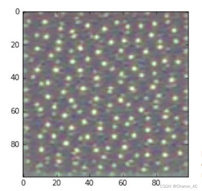

看起来，block3_conv1 层第0个过滤器响应的是波尔卡点(polka-dot)图案。下面来看有趣的部分:可以将每一层的每个过滤器都可视化。为了简单起见，只查看每层的前64个过滤器，并只查看每个卷积块的第一层(即block1_conv1、block2_conv1block3_conv、block4 conv1、block5 conv1)。我们将输出放在一个8x8的网格中每个网格是一个64像素x64 像素的过滤器模式，两个过滤器模式之间留有一些黑边(见图5-30~图5-33)。

"""生成某一层中所有过滤器响应模式组成的网格"""
for layer_name in ['block1_conv1', 'block2_conv1', 'block3_conv1', 'block4_conv1']:
    size = 64
    margin = 5

    # This a empty (black) image where we will store our results.
    """空图像（全黑色），用于保存结果"""
    results = np.zeros((8 * size + 7 * margin, 8 * size + 7 * margin, 3))

    for i in range(8):  # iterate over the rows of our results grid
        for j in range(8):  # iterate over the columns of our results grid
            # Generate the pattern for filter `i + (j * 8)` in `layer_name`
            """生成layer_name层第i+（j+8）个过滤器的模式"""
            filter_img = generate_pattern(layer_name, i + (j * 8), size=size)

            # Put the result in the square `(i, j)` of the results grid
            """将结果放入results网格第(i,j)个方块中"""
            horizontal_start = i * size + i * margin
            horizontal_end = horizontal_start + size
            vertical_start = j * size + j * margin
            vertical_end = vertical_start + size
            results[horizontal_start: horizontal_end, vertical_start: vertical_end, :] = filter_img

    # Display the results grid
    """显示results网格"""
    plt.figure(figsize=(20, 20))
    plt.imshow(results)
    plt.show()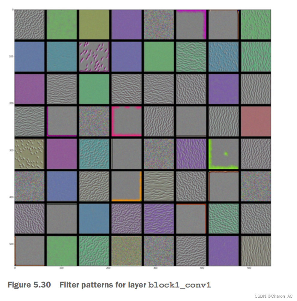

图5-30 block1_conv1层的过滤器模式

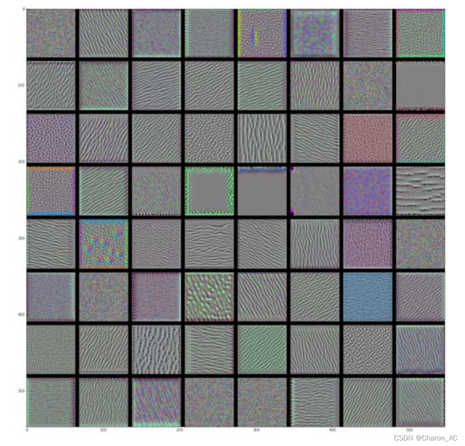
图5-31 block2_conv1 层的过滤器模式

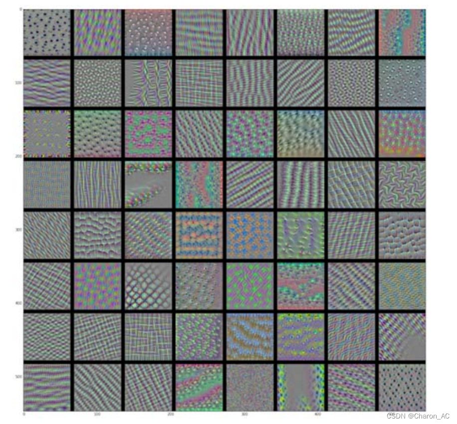
图5-32 block3_conv1 层的过滤器模式

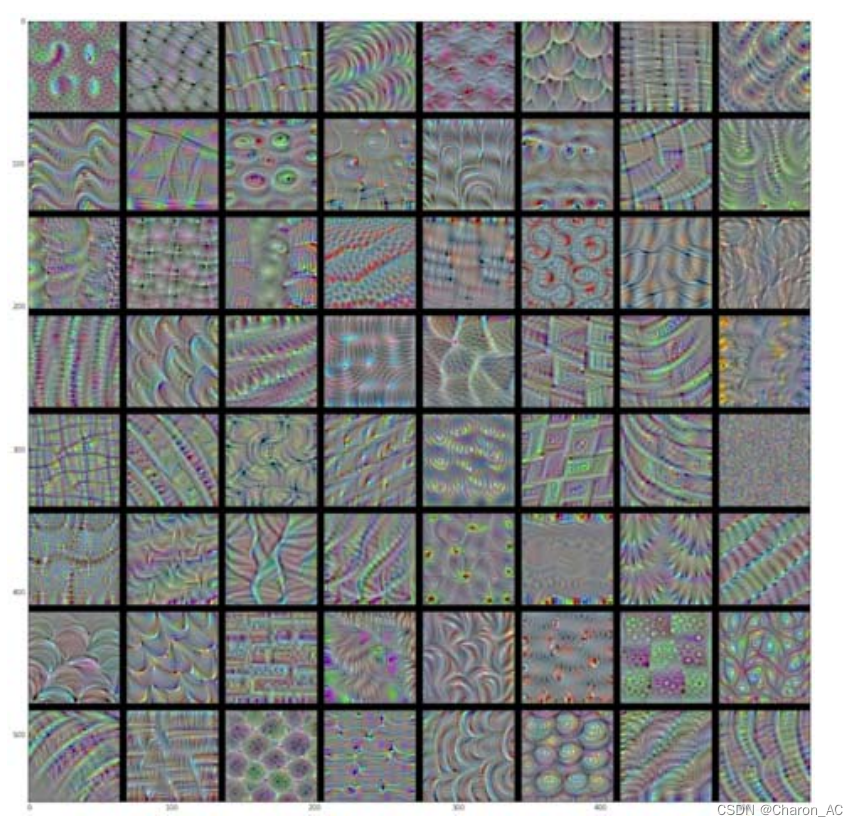 图5-33 block4_conv1 层的过滤器模式

这些过滤器可视化包含卷积神经网络的层如何观察世界的很多信息:卷积神经网络中每层都学习一组过滤器，以便将其输人表示为过滤器的组合。这类似于傅里叶变换将信号分解为-组余弦函数的过程。随着层数的加深，卷积神经网络中的过滤器变得越来越复杂，越来越精细口

        模型第一层(block1_conv1)的过滤器对应简单的方向边缘和颜色(还有一些是彩色边缘)。
        block2_conv1 层的过滤器对应边缘和颜色组合而成的简单纹理口

        更高层的过滤器类似于自然图像中的纹理:羽毛、眼睛、树叶等。

3.可视化类激活的热力图

介绍另一种可视化方法，它有助于了解一张图像的哪一部分让卷积神经网络做出了最终的分类决策。这有助于对卷积神经网络的决策过程进行调试,特别是出现分类错误的情况下这种方法还可以定位图像中的特定目标。
这种通用的技术叫作类激活图(CAM，class activation map)可视化，它是指对输入图像生成类激活的热力图。类激活热力图是与特定输出类别相关的二维分数网格，对任何输人图像的每个位置都要进行计算，它表示每个位置对该类别的重要程度。举例来说，对于输入到猫狗分类卷积神经网络的一张图像，CAM可视化可以生成类别“猫”的热力图，表示图像的各个部分与“猫”的相似程度，CAM 可视化也会生成类别“狗”的热力图，表示图像的各个部分与“狗的相似程度。
我们将使用的具体实现方式是“Grad-CAM: visualexplanations from deep networks via gradient-basedlocalization”@这篇论文中描述的方法。这种方法非常简单:给定一张输入图像，对于一个卷积层的输出特征图，用类别相对于通道的梯度对这个特征图中的每个通道进行加权。直观上来看，理解这个技巧的一种方法是，你是用“每个通道对类别的重要程度”对“输入图像对不同通道的激活强度”的空间图进行加权，从而得到了“输人图像对类别的激活强度”的空间图。我们再次使用预训练的VGG16网络来演示此方法

"""加载带有预训练权重的VGG16网格"""
from keras.applications.vgg16 import VGG16

K.clear_session()

# Note that we are including the densely-connected classifier on top;
# all previous times, we were discarding it.
"""注意，网络中包括了密集连接器。在前面所有的例子中，都舍弃了这个分类器"""
model = VGG16(weights='imagenet')

图 5-34 显示了两只非洲象的图像，可能是一只母象和它的小象，它们在大草原上漫步。我们将这张图像转换为 VGG16 模型能够读取的格式:模型在大小为224x224 的图像上进行训练，这些训练图像都根据 keras.applications.vgg16.preprocess.input 函数中内置的规则进行预处理。因此，我们需要加载图像，将其大小调整为 224x224然后将其转换为 float32格式的Numpy 张量，并应用这些预处理规则。

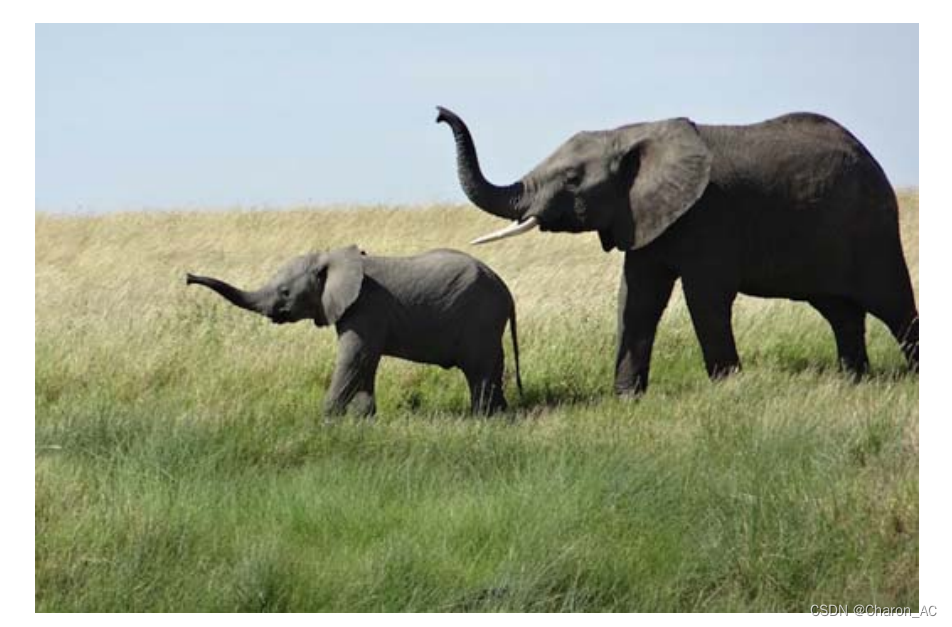
图5-34非洲象的测试图像

"""为VGG16模型预处理一张输入图像"""
from keras.preprocessing import image
from keras.applications.vgg16 import preprocess_input, decode_predictions
import numpy as np

# The local path to our target image
"""目标图像的本地路径"""
img_path = '/Users/fchollet/Downloads/creative_commons_elephant.jpg'

# `img` is a PIL image of size 224x224
"""大小为224*224的python图像库"""
img = image.load_img(img_path, target_size=(224, 224))

# `x` is a float32 Numpy array of shape (224, 224, 3)
"""形状为（224,224,3）的float32格式的numpy数组"""
x = image.img_to_array(img)

# We add a dimension to transform our array into a "batch"
# of size (1, 224, 224, 3)
"""添加一个维度，将数组转化为（1,224,224,3）形状的批量"""
x = np.expand_dims(x, axis=0)

# Finally we preprocess the batch
# (this does channel-wise color normalization)
"""对批量进行预处理（按通道进行颜色标准化）"""
x = preprocess_input(x)


"""运行一下"""
preds = model.predict(x)
print('Predicted:', decode_predictions(preds, top=3)[0])
Predicted: [('n02504458', 'African_elephant', 0.90942144), ('n01871265', 'tusker', 0.08618243), ('n02504013', 'Indian_elephant', 0.0043545929)]

"""对这张图像预测的前三个类别分别为:
非洲象(African elephant，92.5%的概率)
口长牙动物(tusker，7%的概率)
印度象(Indian elephant，0.4%的概率)
网络识别出图像中包含数量不确定的非洲象。预测向量中被最大激活的元素是对应“非洲象类别的元素，索引编号为386。"""


np.argmax(preds[0])
386




"""为了展示图像中哪些部分最像非洲象，我们来使用Grad-CAM算法。"""
"""应用Grad-CAM算法"""

# This is the "african elephant" entry in the prediction vector
"""预测向量中的“非洲象”元素"""
african_elephant_output = model.output[:, 386]

# The is the output feature map of the `block5_conv3` layer,
# the last convolutional layer in VGG16
"""block5_conv3层的输出特征图它是VGG16的最后一个卷积层"""
last_conv_layer = model.get_layer('block5_conv3')

# This is the gradient of the "african elephant" class with regard to
# the output feature map of `block5_conv3`
"""“非洲象”类别相对于block5_conv3输出特征图的梯度"""
grads = K.gradients(african_elephant_output, last_conv_layer.output)[0]

# This is a vector of shape (512,), where each entry
# is the mean intensity of the gradient over a specific feature map channel
"""形状为(512，)的向量，每个元素是特定特征图通道的梯度平均大小"""
pooled_grads = K.mean(grads, axis=(0, 1, 2))

# This function allows us to access the values of the quantities we just defined:
# `pooled_grads` and the output feature map of `block5_conv3`,
# given a sample image
"""访问刚刚定义的量:对于给定的样本图像，pooled_grads 和 block5_conv3 层的输出特征图"""
iterate = K.function([model.input], [pooled_grads, last_conv_layer.output[0]])

# These are the values of these two quantities, as Numpy arrays,
# given our sample image of two elephants
"""对于两个大象的样本图像这两个量都是Numpy数组"""
pooled_grads_value, conv_layer_output_value = iterate([x])

# We multiply each channel in the feature map array
# by "how important this channel is" with regard to the elephant class
"""将特征图数组的每个通道乘以“这个通道对“大象’类别的重要程度”"""
for i in range(512):
    conv_layer_output_value[:, :, i] *= pooled_grads_value[i]

# The channel-wise mean of the resulting feature map
# is our heatmap of class activation
"""得到的特征图的逐通道平均值即为类激活的热力图"""
heatmap = np.mean(conv_layer_output_value, axis=-1)



"""为了便于可视化，我们还需要将热力图标准化到0~1 范围内"""
"""热力图后处理"""
heatmap = np.maximum(heatmap, 0)
heatmap /= np.max(heatmap)
plt.matshow(heatmap)
plt.show()

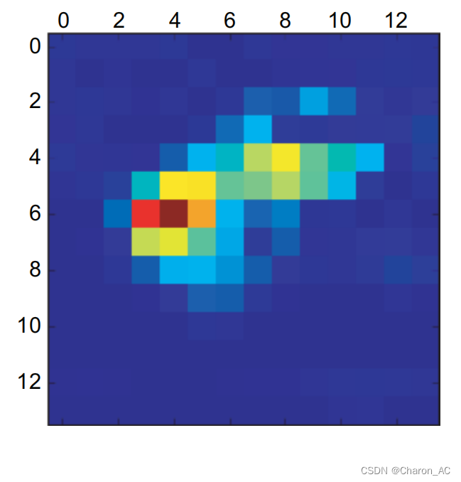
图5-35测试图像的“非洲象”类激活热力图

最后用 OpenCV 来生成一张图像，将原始图像叠加在刚刚得到的热力图上(见图 5-36)。

"""将热力图和原始图像叠加"""
import cv2

# We use cv2 to load the original image
"""用cv2加载原始图像"""
img = cv2.imread(img_path)

# We resize the heatmap to have the same size as the original image
"""将热力图的大小调整为与原始图像相同"""
heatmap = cv2.resize(heatmap, (img.shape[1], img.shape[0]))

# We convert the heatmap to RGB
"""将热力图转化为RGB格式"""
heatmap = np.uint8(255 * heatmap)

# We apply the heatmap to the original image
"""将热力图应用于原始图像"""
heatmap = cv2.applyColorMap(heatmap, cv2.COLORMAP_JET)

# 0.4 here is a heatmap intensity factor
"""这里0.4是热力图强度因子"""
superimposed_img = heatmap * 0.4 + img

# Save the image to disk
"""将图像保存到硬盘"""
cv2.imwrite('/Users/fchollet/Downloads/elephant_cam.jpg', superimposed_img)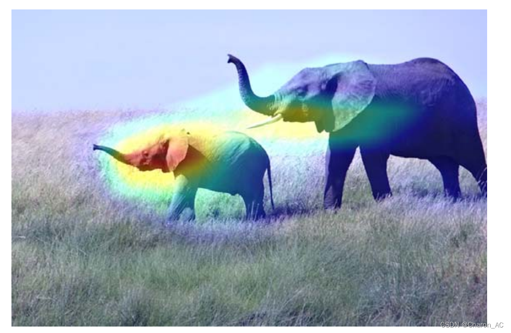

 

图5-36 将类激活热力图叠加到原始图像上

这种可视化方法回答了两个重要问题:
网络为什么会认为这张图像中包含一头非洲象?
 非洲象在图像中的什么位置?
尤其值得注意的是，小象耳朵的激活强度很大，这可能是网络找到的非洲象和印度象的不同之处。 

小结

卷积神经网络是解决视觉分类问题的最佳工具。
卷积神经网络通过学习模块化模式和概念的层次结构来表示视觉世界

卷积神经网络学到的表示很容易可视化，卷积神经网络不是黑盒。

现在能够从头开始训练自己的卷积神经网络来解决图像分类问题

知道了如何使用视觉数据增强来防止过拟合。
知道了如何使用预训练的卷积神经网络进行特征提取与模型微调。

可以将卷积神经网络学到的过滤器可视化，也可以将类激活热力图可视化