R语言逻辑回归与lasso模型

一、数据描述

数据集heart_learning.csv与heart_test.csv是关于心脏病的数据集，heart_learning.csv是训练数据集，heart_test.csv是测试数据集。

变量名称	变量说明
age	年龄
sex	性别，取值1代表男性，0代表女性
pain	胸痛的类型，取值1,2,3,4,代表4种类型
bpress	入院时的静息血压（单位：毫米汞柱
chol	血清胆固醇（单位：毫克/分升
bsugar	空腹血糖是否大于120毫克/公升，1代表是，0代表否
ekg	静息心电图结果，取值0,1,2代表3中不同的结果
thalach	达到的最大心率
exang	是否有运动性心绞痛，1代表是0代表否
oldpeak	运动引起的ST段压低
slope	锻炼高峰期ST段的斜率，取值1代表上斜，2代表平坦，3代表下斜
ca	荧光染色的大血管数目，取值为0,1,2,3
thal	取值3代表正常，取值6代表固定缺陷，取值7代表可逆缺陷
target	因变量，直径减少50%以上的大血管数目，取值0,1,2,3,4
target2	因变量，取值1表示target大于0，取值0表示target等于0

二、读取数据集

heart_learning<-read.csv('f:/桌面/heart_learning.csv',colClasses = rep('numeric',15))

head(heart_learning)

heart_test<-read.csv('f:/桌面/heart_test.csv',colClasses = rep('numeric',15))

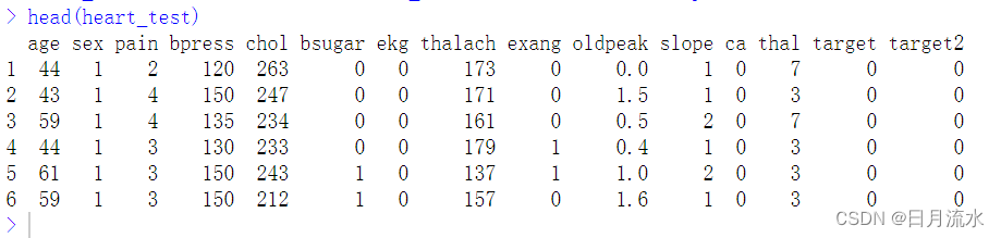
head(heart_test)

三、数据整理

将不是哑变量形式的定类自变量转换为因子变量，在本例中主要转换的变量为pain,ekg,slope,ca,thal,使用管道函数%>%和mutate()将两个数据集的变量进行类型转换。

heart_learning<-heart_learning %>% mutate(pain=as.factor(pain)) %>% mutate(ekg=as.factor(ekg)) %>%mutate(slope=as.factor(slope)) %>% mutate(thal=as.factor(thal))

heart_test<-heart_test %>% mutate(pain=as.factor(pain)) %>% mutate(ekg=as.factor(ekg)) %>% mutate(slope=as.factor(slope)) %>% mutate(thal=as.factor(thal))

转换后：

str(heart_learning)
str(heart_test)

 str(heart_learning)
'data.frame':	206 obs. of  15 variables:
 $ age    : num  63 37 41 56 57 57 56 52 57 54 ...
 $ sex    : num  1 1 0 1 0 1 0 1 1 1 ...
 $ pain   : Factor w/ 4 levels "1","2","3","4": 1 3 2 2 4 4 2 3 3 4 ...
 $ bpress : num  145 130 130 120 120 140 140 172 150 140 ...
 $ chol   : num  233 250 204 236 354 192 294 199 168 239 ...
 $ bsugar : num  1 0 0 0 0 0 0 1 0 0 ...
 $ ekg    : Factor w/ 3 levels "0","1","2": 3 1 3 1 1 1 3 1 1 1 ...
 $ thalach: num  150 187 172 178 163 148 153 162 174 160 ...
 $ exang  : num  0 0 0 0 1 0 0 0 0 0 ...
 $ oldpeak: num  2.3 3.5 1.4 0.8 0.6 0.4 1.3 0.5 1.6 1.2 ...
 $ slope  : Factor w/ 3 levels "1","2","3": 3 3 1 1 1 2 2 1 1 1 ...
 $ ca     : num  0 0 0 0 0 0 0 0 0 0 ...
 $ thal   : Factor w/ 3 levels "3","6","7": 2 1 1 1 1 2 1 3 1 1 ...
 $ target : num  0 0 0 0 0 0 0 0 0 0 ...
 $ target2: num  0 0 0 0 0 0 0 0 0 0 ...

 str(heart_test)
'data.frame':	91 obs. of  15 variables:
 $ age    : num  44 43 59 44 61 59 44 65 51 45 ...
 $ sex    : num  1 1 1 1 1 1 1 0 0 1 ...
 $ pain   : num  2 4 4 3 3 3 2 3 3 4 ...
 $ bpress : num  120 150 135 130 150 150 130 155 140 104 ...
 $ chol   : num  263 247 234 233 243 212 219 269 308 208 ...
 $ bsugar : num  0 0 0 0 1 1 0 0 0 0 ...
 $ ekg    : num  0 0 0 0 0 0 2 0 2 2 ...
 $ thalach: num  173 171 161 179 137 157 188 148 142 148 ...
 $ exang  : num  0 0 0 1 1 0 0 0 0 1 ...
 $ oldpeak: num  0 1.5 0.5 0.4 1 1.6 0 0.8 1.5 3 ...
 $ slope  : num  1 1 2 1 2 1 1 1 1 2 ...
 $ ca     : num  0 0 0 0 0 0 0 0 1 0 ...
 $ thal   : num  7 3 7 3 3 3 3 3 3 3 ...
 $ target : num  0 0 0 0 0 0 0 0 0 0 ...
 $ target2: num  0 0 0 0 0 0 0 0 0 0 ...

四、二元逻辑回归

1、建立二元变量target2对自变量age,sex,pain,bpress,chol,bsugar,ekg,thalach,exang,等自变量的回归模型，因为因变量target2仅取0和1两值，因此该模型为普通的logistic逻辑模型。

fit_lm<-glm(target2~.,data=heart_learning[,-14],family = 'binomial')

summary(fit_lm)

summary(fit_lm)

Call:
glm(formula = target2 ~ ., family = "binomial", data = heart_learning[, 
    -14])

Coefficients:
              Estimate Std. Error z value Pr(>|z|)   
(Intercept) -6.079e+00  3.764e+00  -1.615  0.10634   
age         -2.382e-02  3.151e-02  -0.756  0.44975   
sex          1.771e+00  6.958e-01   2.545  0.01091 * 
pain2        1.144e+00  9.911e-01   1.154  0.24837   
pain3        5.378e-01  8.215e-01   0.655  0.51267   
pain4        2.277e+00  8.550e-01   2.663  0.00774 **
bpress       4.034e-02  1.517e-02   2.658  0.00786 **
chol         8.330e-03  5.616e-03   1.483  0.13804   
bsugar      -6.162e-01  8.091e-01  -0.762  0.44631   
ekg1         1.376e+01  1.587e+03   0.009  0.99309   
ekg2         8.554e-01  5.142e-01   1.664  0.09619 . 
thalach     -3.648e-02  1.502e-02  -2.428  0.01516 * 
exang        7.524e-01  5.533e-01   1.360  0.17385   
oldpeak      6.505e-01  3.237e-01   2.010  0.04446 * 
slope2       4.972e-01  6.077e-01   0.818  0.41329   
slope3      -4.059e-01  1.358e+00  -0.299  0.76504   
ca           9.082e-01  3.277e-01   2.772  0.00558 **
thal6        9.011e-02  1.181e+00   0.076  0.93920   
thal7        1.639e+00  5.651e-01   2.901  0.00372 **
---
Signif. codes:  0 ‘***’ 0.001 ‘**’ 0.01 ‘*’ 0.05 ‘.’ 0.1 ‘ ’ 1

(Dispersion parameter for binomial family taken to be 1)

    Null deviance: 284.00  on 205  degrees of freedom
Residual deviance: 121.07  on 187  degrees of freedom
AIC: 159.07

Number of Fisher Scoring iterations: 15

运行得到了回归模型的系数。

2、将在训练数据集中得到的逻辑回归模型运用到测试数据，用以检验模型的拟合情况。

test.pred<-predict(fit_lm,heart_test,type = 'response')

head(test.pred)

type = 'response'表明拟合的类型为因变量target2取值为1的概率。

 head(test.pred)
         1          2          3          4          5          6 
0.13562868 0.44796749 0.63351630 0.04108158 0.29696382 0.06530277 

test.pred.class<-1*(test.pred>0.5)

test.pred.class

表明当因变量target2预测的概率取值大于0.5是，该target2就取值为1，反之小于0.5时则取值为0.

运行得到预测的分类取值，

 test.pred.class
 1  2  3  4  5  6  7  8  9 10 11 12 13 14 15 16 17 18 19 20 21 22 23 24 25 26 27 28 29 30 31 32 33 34 35 36 37 38 39 
 0  0  1  0  0  0  0  0  0  1  0  0  0  0  0  0  0  0  0  0  0  0  0  1  0  0  1  0  0  0  0  0  0  0  0  0  0  0  0 
40 41 42 43 44 45 46 47 48 49 50 51 52 53 54 55 56 57 58 59 60 61 62 63 64 65 66 67 68 69 70 71 72 73 74 75 76 77 78 
 0  0  1  1  0  1  0  0  0  0  0  1  1  0  1  1  0  1  1  1  0  0  0  1  0  0  1  1  1  1  1  1  1  1  0  1  1  1  1 
79 80 81 82 83 84 85 86 87 88 89 90 91 
 1  1  1  1  1  1  1  1  1  1  1  1  1 

table(heart_test$target2,test.pred.class)

则得到了真实的分类取值和预测值的列联表

table(heart_test$target2,test.pred.class)
   test.pred.class
     0  1
  0 41  7
  1 10 33

五、多值逻辑变量回归

1、即要求因变量taregt对自变量age,sex,pain,bpress等自变量进行回归分析，因变量target取值为0,1,2,3,4这5个取值。

library(MASS)

fit.ologit <- polr(as.factor(target) ~ ., data=heart_learning[,-15])

summary(fit.ologit)模型的系数

summary(fit.ologit)

Re-fitting to get Hessian

Call:
polr(formula = as.factor(target) ~ ., data = heart_learning[, 
    -15])

Coefficients:
            Value Std. Error  t value
age     -0.014686   0.021748 -0.67527
sex      0.909686   0.432821  2.10176
pain2    0.618309   0.839876  0.73619
pain3    0.406543   0.729413  0.55736
pain4    1.668044   0.722760  2.30788
bpress   0.026835   0.010207  2.62913
chol     0.002481   0.003297  0.75255
bsugar  -0.190277   0.495656 -0.38389
ekg1     1.303400   1.270044  1.02626
ekg2     0.658572   0.338254  1.94697
thalach -0.026755   0.009609 -2.78448
exang    0.312088   0.380035  0.82121
oldpeak  0.262455   0.176701  1.48530
slope2   0.596782   0.427343  1.39650
slope3   0.078796   0.860779  0.09154
ca       0.666761   0.201982  3.30109
thal6    1.030344   0.785958  1.31094
thal7    1.496852   0.404164  3.70357

Intercepts:
    Value   Std. Error t value
0|1  3.2295  2.4368     1.3253
1|2  5.0011  2.4493     2.0418
2|3  6.2313  2.4554     2.5378
3|4  8.1594  2.4755     3.2960

Residual Deviance: 355.4983 
AIC: 399.4983 

2、将使用训练数据集中得到的模型运用到测试数据集，以验证模型的拟合预测情况

prob.ologit <- predict(fit.ologit, heart_test, type="probs")
head(prob.ologit)

head(prob.ologit)
          0          1           2           3            4
1 0.8329684 0.13405365 0.023110414 0.008420372 0.0014471768
2 0.6956545 0.23509494 0.047970289 0.018128313 0.0031519743
3 0.3538205 0.40919462 0.153773047 0.070184478 0.0130273377
4 0.9460872 0.04431458 0.006774099 0.002412405 0.0004116821
5 0.7037903 0.22941377 0.046307360 0.017455939 0.0030326152
6 0.9002005 0.08129427 0.013025629 0.004678986 0.0008006112

运行得到了因变量在每个样本观测中的取各种值的概率。

class.ologit <- predict(fit.ologit, heart_test, type="class")
class.ologit

运行得到了模型的预测分类取值情况。

class.ologit <- predict(fit.ologit, heart_test, type="class")
> class.ologit
 [1] 0 0 1 0 0 0 0 0 0 0 0 0 0 0 0 0 0 0 0 0 0 0 0 0 0 0 1 0 0 0 0 0 0 0 0 0 0 0 0 0 0 3 0 0 1 0 0 0 0 0 3 1 0 1 1 0
[57] 1 3 3 0 0 0 1 0 0 1 3 3 3 3 1 3 0 0 3 1 1 3 1 3 1 4 1 3 3 1 4 3 1 1 3
Levels: 0 1 2 3 4

table(heart_test$target, class.ologit)

运行得到了测试数据的实际取值情况和模型预测的取值的列联表。

  class.ologit
     0  1  2  3  4
  0 44  3  0  1  0
  1  9  5  0  3  0
  2  2  3  0  6  0
  3  0  5  0  4  2
  4  0  2  0  2  0

六、将Lasso模型运用到二元逻辑模型。

此时模型的因变为target2,取1和0二值。

library(glmnet)

library(caret)

1、将分类变量转换为哑变量

dmy <- dummyVars(~pain+ekg+slope+thal,
                 heart_learning, 
                 fullRank = TRUE)

2、将哑变量加进原始数据集中，并去除多余变量

heart_learning2 <- cbind(heart_learning,predict(dmy,heart_learning)) %>%  dplyr::select(-c(pain,ekg,slope,thal)) %>% dplyr:: select(-c(target,target2),everything())

str(heart_learning2)

str(heart_learning2)
'data.frame':	206 obs. of  20 variables:
 $ age    : num  63 37 41 56 57 57 56 52 57 54 ...
 $ sex    : num  1 1 0 1 0 1 0 1 1 1 ...
 $ bpress : num  145 130 130 120 120 140 140 172 150 140 ...
 $ chol   : num  233 250 204 236 354 192 294 199 168 239 ...
 $ bsugar : num  1 0 0 0 0 0 0 1 0 0 ...
 $ thalach: num  150 187 172 178 163 148 153 162 174 160 ...
 $ exang  : num  0 0 0 0 1 0 0 0 0 0 ...
 $ oldpeak: num  2.3 3.5 1.4 0.8 0.6 0.4 1.3 0.5 1.6 1.2 ...
 $ ca     : num  0 0 0 0 0 0 0 0 0 0 ...
 $ pain2  : num  0 0 1 1 0 0 1 0 0 0 ...
 $ pain3  : num  0 1 0 0 0 0 0 1 1 0 ...
 $ pain4  : num  0 0 0 0 1 1 0 0 0 1 ...
 $ ekg1   : num  0 0 0 0 0 0 0 0 0 0 ...
 $ ekg2   : num  1 0 1 0 0 0 1 0 0 0 ...
 $ slope2 : num  0 0 0 0 0 1 1 0 0 0 ...
 $ slope3 : num  1 1 0 0 0 0 0 0 0 0 ...
 $ thal6  : num  1 0 0 0 0 1 0 0 0 0 ...
 $ thal7  : num  0 0 0 0 0 0 0 1 0 0 ...
 $ target : num  0 0 0 0 0 0 0 0 0 0 ...
 $ target2: num  0 0 0 0 0 0 0 0 0 0 ...

3、建立lasso模型

fit.lasso <- glmnet(as.matrix(heart_learning2[,1:18]),
                         heart_learning2$target2, 
                         family="binomial")

fit.lasso

 Df  %Dev   Lambda
1   0  0.00 0.268700
2   2  3.89 0.244800
3   2  8.32 0.223100
4   3 12.46 0.203300
5   4 16.55 0.185200
6   4 20.23 0.168800
7   4 23.40 0.153800
8   6 26.51 0.140100
9   6 29.30 0.127700
10  6 31.75 0.116300
11  6 33.90 0.106000
12  6 35.79 0.096570
13  7 37.48 0.087990
14  7 39.01 0.080170
15  7 40.37 0.073050
16  8 41.58 0.066560
17  9 42.87 0.060650
18  9 44.22 0.055260
19 10 45.44 0.050350
20 10 46.60 0.045880
21 10 47.64 0.041800
22 10 48.56 0.038090
23 10 49.38 0.034710
24 11 50.15 0.031620
25 11 50.88 0.028810
26 11 51.53 0.026250
27 11 52.11 0.023920
28 11 52.62 0.021800
29 11 53.08 0.019860
30 12 53.50 0.018100
31 12 53.90 0.016490
32 12 54.26 0.015020
33 12 54.57 0.013690
34 12 54.84 0.012470
35 12 55.08 0.011360
36 12 55.29 0.010350
37 13 55.47 0.009435
38 15 55.67 0.008597
39 16 55.86 0.007833
40 16 56.05 0.007137
41 16 56.22 0.006503
42 16 56.36 0.005925
43 16 56.48 0.005399
44 16 56.58 0.004919
45 16 56.67 0.004482
46 16 56.75 0.004084
47 17 56.82 0.003721
48 17 56.90 0.003391
49 17 56.97 0.003090
50 17 57.03 0.002815
51 17 57.08 0.002565
52 17 57.13 0.002337
53 17 57.16 0.002130
54 18 57.19 0.001940
55 18 57.22 0.001768
56 18 57.24 0.001611
57 18 57.26 0.001468
58 18 57.28 0.001337
59 18 57.29 0.001219
60 18 57.30 0.001110
61 18 57.31 0.001012
62 18 57.32 0.000922
63 18 57.33 0.000840
64 18 57.33 0.000765
65 18 57.34 0.000697
66 18 57.34 0.000635
67 18 57.35 0.000579
68 18 57.35 0.000527
69 18 57.35 0.000481
70 18 57.36 0.000438
71 18 57.36 0.000399
72 18 57.36 0.000364
73 18 57.36 0.000331
74 18 57.36 0.000302
75 18 57.36 0.000275
76 18 57.36 0.000251

运行得到每次运行处理结果情况。

根据该模型，参数λ为调节参数，当λ逐渐增大是，所有模型系数都将趋于0，所有参数λ常用于变量选择。从图形中可以看到随着对数的λ值逐渐增大，每个变量代表的系数也逐渐趋于0.

3、使用交叉验证选取调节参数λ的值得到模型的回归系数

cvfit.lasso <- cv.glmnet(as.matrix(heart_learning2[,1:18]),
                         heart_learning2$target2, 
                         family="binomial", 
                         type.measure="class")

在这里使用了 cv.glmnet()函数，使用交叉验证选取调节参数的最佳值，因变量为二项分布，交叉验证的准则为错误分类率。

cvfit.lasso$lambda.min

运行得到了交叉验证的λ值为lmbda.min

 cvfit.lasso$lambda.min
[1] 0.02881333

coef(cvfit.lasso,s='lambda.min')

运行得到了模型的系数：

coef(cvfit.lasso,s='lambda.min')
19 x 1 sparse Matrix of class "dgCMatrix"
                       s1
(Intercept) -1.6734148389
age          .           
sex          0.5478601756
bpress       0.0123146239
chol         0.0005767132
bsugar       .           
thalach     -0.0184055035
exang        0.5116235150
oldpeak      0.3216762530
ca           0.4622937819
pain2        .           
pain3        .           
pain4        1.0975807443
ekg1         .           
ekg2         0.2317211271
slope2       0.2993419586
slope3       .           
thal6        .           
thal7        1.2936765301

上述系数中，没有显示系数值的变量将被剔除。

plot(cvfit.lasso)

运行得到：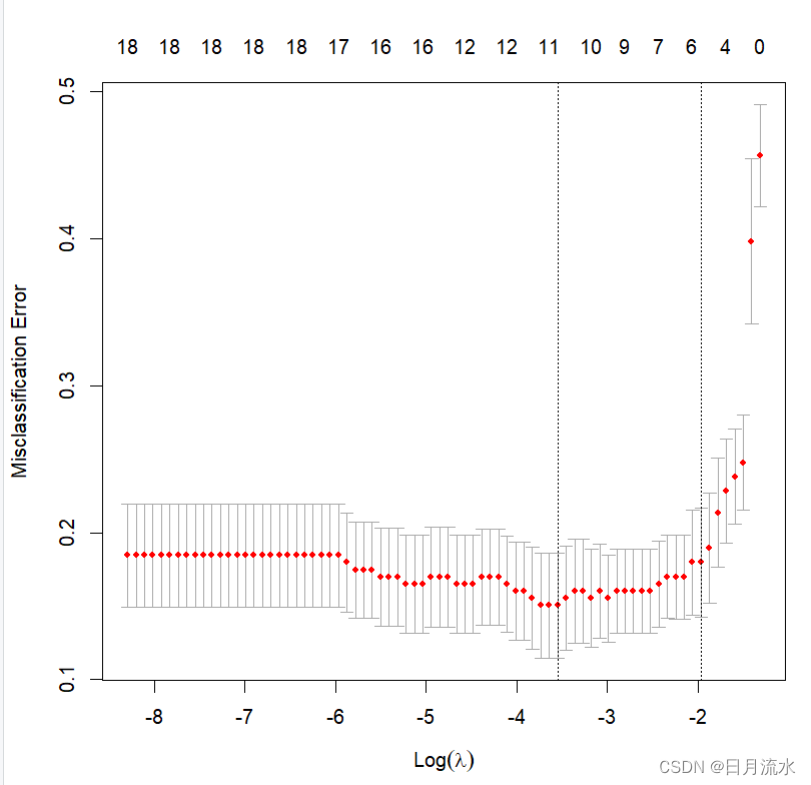

交叉验证的平均误差随着调节参数lambd对数值的变化而变化的图形，从图形中交叉验证的平均误差最小值对于的lambda,对数为-3.546917，相应的lambda的值为 0.02881333。从图形中最上面的对应数值看到，相应的选择进入模型变量为11个。

4、测试数据的拟合验证

heart_test2 <- 
  cbind(heart_test,predict(dmy,heart_test)) %>%  dplyr::select(-c(pain,ekg,slope,thal)) %>% 
  dplyr::select(-c(target,target2),everything())
prob.lasso <-
  predict(cvfit.lasso, as.matrix(heart_test2[,1:18]), 
          s="lambda.min", type="response")

对测试数据集进行整理，在整理后数据集进行进行lasso模型的拟合，得到因变量的概率取值的预测。

head(prob.lasso)
  lambda.min
1  0.1999511
2  0.3311122
3  0.6364576
4  0.1146022
5  0.3711861
6  0.1778357

class.lasso <- 
  predict(cvfit.lasso, as.matrix(heart_test2[,1:18]), 
          s="lambda.min", type="class")
head(class.lasso)

运行得到了因变量的取值情况

head(class.lasso)
  lambda.min
1 "0"       
2 "0"       
3 "1"       
4 "0"       
5 "0"       
6 "0

table(heart_test$target2, class.lasso)

运行得到了因变量真实值和预测值的列联表。

table(heart_test$target2, class.lasso)
   class.lasso
     0  1
  0 43  5
  1 10 33

七、将Lasso模型运用到多值逻辑模型

相应的程序为：

cvfit2.lasso <- cv.glmnet(as.matrix(heart_learning2[,1:18]),
                         heart_learning2$target, 
                         family="multinomial", 
                         type.measure="class")

prob2.lasso <- predict(cvfit2.lasso, as.matrix(heart_test2[,1:18]), 
          s="lambda.min", type="response")

head(prob2.lasso)

得到：

head(prob2.lasso)
, , 1

          0          1          2          3          4
1 0.7819545 0.12867778 0.03665610 0.03401131 0.01870034
2 0.6889450 0.14948312 0.08312511 0.05084087 0.02760589
3 0.3670365 0.32374751 0.15268963 0.10556503 0.05096128
4 0.8866576 0.06487749 0.01947599 0.01893834 0.01005056
5 0.6836868 0.13274797 0.06431920 0.08618101 0.03306503
6 0.8531171 0.06231089 0.03283587 0.03465448 0.01708167

得到因变量取值的概率

class2.lasso <-  predict(cvfit2.lasso, as.matrix(heart_test2[,1:18]), 
          s="lambda.min", type="class")

得到了因变的预测值

head(class2.lasso)
     1  
[1,] "0"
[2,] "0"
[3,] "0"
[4,] "0"
[5,] "0"
[6,] "0"

table(heart_test2$target, class2.lasso)

因变量真实值和预测值列联表：

table(heart_test2$target, class2.lasso)
   class2.lasso
     0  1  2  3
  0 45  2  1  0
  1 12  3  2  0
  2  2  5  2  2
  3  2  6  1  2
  4  1  1  1  1

本文结束。