2024年最新可分离卷积及深度可分离卷积详解_深度卷积和深度可分离卷积(1)，2024年展望Linux运维原生开发的现状

2301_79054215

已于 2024-05-09 19:19:20 修改

阅读量312

点赞数 4

分类专栏：程序员文章标签：运维 linux 服务器

于 2024-05-09 19:19:18 首次发布

本文链接：https://blog.csdn.net/2301_79054215/article/details/138627705

版权

程序员专栏收录该内容

135 篇文章 0 订阅

订阅专栏

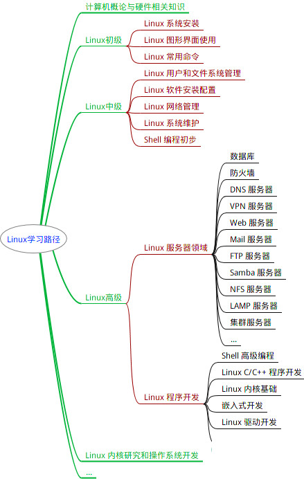
最全的Linux教程，Linux从入门到精通

======================

linux从入门到精通(第2版)
Linux系统移植
Linux驱动开发入门与实战
LINUX 系统移植第2版
Linux开源网络全栈详解从DPDK到OpenFlow

华为18级工程师呕心沥血撰写3000页Linux学习笔记教程

第一份《Linux从入门到精通》466页

====================

内容简介

====

本书是获得了很多读者好评的Linux经典畅销书**《Linux从入门到精通》的第2版**。本书第1版出版后曾经多次印刷，并被51CTO读书频道评为“最受读者喜爱的原创IT技术图书奖”。本书第﹖版以最新的Ubuntu 12.04为版本，循序渐进地向读者介绍了Linux 的基础应用、系统管理、网络应用、娱乐和办公、程序开发、服务器配置、系统安全等。本书附带1张光盘，内容为本书配套多媒体教学视频。另外,本书还为读者提供了大量的Linux学习资料和Ubuntu安装镜像文件，供读者免费下载。

华为18级工程师呕心沥血撰写3000页Linux学习笔记教程

本书适合广大Linux初中级用户、开源软件爱好者和大专院校的学生阅读，同时也非常适合准备从事Linux平台开发的各类人员。

需要《Linux入门到精通》、《linux系统移植》、《Linux驱动开发入门实战》、《Linux开源网络全栈》电子书籍及教程的工程师朋友们劳烦您转发+评论

网上学习资料一大堆，但如果学到的知识不成体系，遇到问题时只是浅尝辄止，不再深入研究，那么很难做到真正的技术提升。

需要这份系统化的资料的朋友，可以点击这里获取！

一个人可以走的很快，但一群人才能走的更远！不论你是正从事IT行业的老鸟或是对IT行业感兴趣的新人，都欢迎加入我们的的圈子（技术交流、学习资源、职场吐槽、大厂内推、面试辅导），让我们一起学习成长！

print(summary(conv, input_size=(3, 64, 64)))

    Layer (type)               Output Shape         Param #

================================================================
Conv2d-1 [-1, 4, 64, 64] 12

Total params: 12
Trainable params: 12
Non-trainable params: 0

Input size (MB): 0.05
Forward/backward pass size (MB): 0.12
Params size (MB): 0.00
Estimated Total Size (MB): 0.17

None


### 2. 分组卷积、深度可分离卷积对比：


* 普通卷积：总参数量是 4x8x3x3=288。
* 分组卷积：假设输入层为一个大小为64×64像素的彩色图片、in\_channels=4，out\_channels=8,经过2组卷积层，最终输出8个Feature Map，我们可以计算出卷积层的参数数量是 2x8x3x3=144。
* 深度可分离卷积：逐深度卷积的卷积数量是 4x3x3=36, 逐点卷积卷积数量是 1x1x4x8=32，总参数量为68。

#普通卷积层
device = torch.device(‘cuda’ if torch.cuda.is_available() else ‘cpu’)
conv = Conv_test(4, 8, 3, padding=1, groups=1).to(device)
print(summary(conv, input_size=(4, 64, 64)))

    Layer (type)               Output Shape         Param #

================================================================
Conv2d-1 [-1, 8, 64, 64] 288

Total params: 288
Trainable params: 288
Non-trainable params: 0

Input size (MB): 0.06
Forward/backward pass size (MB): 0.25
Params size (MB): 0.00
Estimated Total Size (MB): 0.31

None

分组卷积层，输入的是4x64x64,目标输出8个feature map

device = torch.device(‘cuda’ if torch.cuda.is_available() else ‘cpu’)
conv = Conv_test(4, 8, 3, padding=1, groups=2).to(device)
print(summary(conv, input_size=(4, 64, 64)))

    Layer (type)               Output Shape         Param #

================================================================
Conv2d-1 [-1, 8, 64, 64] 144

Total params: 144
Trainable params: 144
Non-trainable params: 0

Input size (MB): 0.06
Forward/backward pass size (MB): 0.25
Params size (MB): 0.00
Estimated Total Size (MB): 0.31

None

逐深度卷积层，输入同上

device = torch.device(‘cuda’ if torch.cuda.is_available() else ‘cpu’)
conv = Conv_test(4, 4, 3, padding=1, groups=4).to(device)
print(summary(conv, input_size=(4, 64, 64)))

    Layer (type)               Output Shape         Param #

================================================================
Conv2d-1 [-1, 4, 64, 64] 36

Total params: 36
Trainable params: 36
Non-trainable params: 0

Input size (MB): 0.06
Forward/backward pass size (MB): 0.12
Params size (MB): 0.00
Estimated Total Size (MB): 0.19

None

逐点卷积层，输入即逐深度卷积的输出大小，目标输出也是8个feature map

device = torch.device(‘cuda’ if torch.cuda.is_available() else ‘cpu’)
conv = Conv_test(4, 8, kernel_size=1, padding=0, groups=1).to(device)
print(summary(conv, input_size=(4, 64, 64)))

    Layer (type)               Output Shape         Param #

================================================================
Conv2d-1 [-1, 8, 64, 64] 32

Total params: 32
Trainable params: 32
Non-trainable params: 0

Input size (MB): 0.06
Forward/backward pass size (MB): 0.25
Params size (MB): 0.00
Estimated Total Size (MB): 0.31

None


### 3. MobileNet V1



![](https://img-blog.csdnimg.cn/2020071700070193.png)

V1这篇文章是17年的提出的一个轻量级神经网络。一句话概括：MobileNetV1就是把VGG中的**标准卷积层**换成**深度可分离卷积**。



> 
> 这种方法能用更少的参数、更少的运算，达到跟跟普通卷差不多的结果。
> 
> 
> 


#### 3.1 MobileNetV1与普通卷积：


**大致结构对比：**



![](https://img-blog.csdnimg.cn/202007170007411.png)
 上图左边是标准卷积层，右边是V1的卷积层。V1的卷积层，首先使用3×3的深度卷积提取特征，接着是一个BN层，随后是一个 
ReLU6，在之后就会逐点卷积，最后就是BN和ReLU了。 
**卷积过程对比：**



![](https://img-blog.csdnimg.cn/20200717000821731.png)

输入尺寸为*D\_f*是输入的特征高度，*D\_w*是输入特征宽度，*M*是输入的channel，*N*是输出的channel。


标准的卷积运算和Depthwise Separable卷积运算计算量的比例为：



![](https://img-blog.csdnimg.cn/20200717000927841.png)

#### 3.2 宽度因子：更薄的模型


如果需要模型更小更快，可以定义一个宽度因子![\alpha](https://private.codecogs.com/gif.latex?%5Calpha)，它可以让网络的每一层都变的更薄。如果input的channel是![M](https://private.codecogs.com/gif.latex?M)就变为![\alpha M](https://private.codecogs.com/gif.latex?%5Calpha%20M)，如果output channel是N就变为![\alpha N](https://private.codecogs.com/gif.latex?%5Calpha%20N)，那么在有宽度因子情况下的深度分离卷积运算的计算量公式就成了如下形式：



![](https://img-blog.csdnimg.cn/2020071700085097.png)

#### 3.3 分辨率因子：减少表达力


分辨率因子![\rho](https://private.codecogs.com/gif.latex?%5Crho)就是减少计算量的超参数，这个因子是和input的长宽相乘，会缩小input的长宽而导致后面的每一层的长宽都缩小。



![](https://img-blog.csdnimg.cn/20200717001053564.png)

#### 3.4 疑惑解答


1. ReLU6：



![](https://img-blog.csdnimg.cn/2020071700114557.png)


![](https://img-blog.csdnimg.cn/20200717001238315.png)

2. 宽度因子和分辨率因子为什么没有出现在V1代码中？

 这是我在看代码时疑惑，因为github上找MobileNetV1的代码官方码是TF的，py给的都是功能块。所以参照官方TF代码可以发现代码对  
 ![\alpha](https://private.codecogs.com/gif.latex?%5Calpha)为0.75，0.5和0.25进行了封装，这样当我们调用模型来构建网络的时候，depth\_multiplier就已经设置为0.75了：

separable_conv2d(
inputs, #size为[batch_size, height, width, channels]的tensor
num_outputs, # 是pointwise卷积运算output的channel，如果为空，就不进行pointwise卷积运算。
kernel_size, #是filter的size [kernel_height, kernel_width]，如果filter的长宽一样可以只填入一个int值。
depth_multiplier, #就是前面介绍过的宽度因子，在代码实现中改成了深度因子，因为是影响的channel，确实深度因子更合适。
stride=1,
padding=‘SAME’,
data_format=DATA_FORMAT_NHWC,
rate=1,
…
)

 关于这两个因子是怎么使用的，代码后面写的是：



![](https://img-blog.csdnimg.cn/20200717001328737.png)


#### 3.5 代码部分相关解释：


`torch.nn.Linear(in_features, out_features, bias=True)`


* *in\_features*：输入特征图的大小
* *out\_features*：输出特征图的大小
* *bias*：如果设置为False，该层不会增加偏差；默认为：True


代码里出现了Sequential，想必我们都不陌生，都知道他是个容器，但我此前并不知道nn.module()里面都包括什么样的“容器”，下面来了解一些常用的：


* `torch.nn.Sequential(*args)`：用于按**顺序**包装一组网络层
* `torch.nn.ModuleList(modules=None)`：用于包装一组网络层，以**迭代**的方式调用网络层
* `torch.nn.ModuleDict(modules=None)`：用于包装一组网络层，以**索引**的方式调用网络层

import torch.nn as nn
import torch.nn.functional as F
from torchsummary import summary

class Block(nn.Module):
‘’‘Depthwise conv + Pointwise conv’‘’
def __init__(self, in_planes, out_planes, stride=1):
super(Block, self).init()
# 深度卷积，通道数不变，用于缩小特征图大小
self.conv1 = nn.Conv2d(in_planes, in_planes, kernel_size=3, stride=stride, padding=1, groups=in_planes, bias=False)
self.bn1 = nn.BatchNorm2d(in_planes)
# 逐点卷积，用于增大通道数
self.conv2 = nn.Conv2d(in_planes, out_planes, kernel_size=1, stride=1, padding=0, bias=False)
self.bn2 = nn.BatchNorm2d(out_planes)

def forward(self, x):
    out = F.relu(self.bn1(self.conv1(x)))
    out = F.relu(self.bn2(self.conv2(out)))
    return out

class MobileNet(nn.Module):
cfg = [
64, (128,2), 128, (256,2), 256, (512,2), 512, 512, 512, 512, 512, (1024,2), 1024
]
def __init__(self, num_classes=10):
super(MobileNet, self).init()
# 首先是一个标准卷积
self.conv1 = nn.Conv2d(3, 32, kernel_size=3, stride=2, padding=1, bias=False)
self.bn1 = nn.BatchNorm2d(32)

    # 然后堆叠深度可分离卷积
    self.layers = self._make_layers(in_planes=32)
 
    self.linear = nn.Linear(1024, num_classes) # 输入的特征图大小为1024，输出特征图大小为10
 
def \_make\_layers(self, in_planes):
    laters = [] #将每层添加到此列表
    for x in self.cfg:
        out_planes = x if isinstance(x, int) else x[0] #isinstance返回的是一个布尔值
        stride = 1 if isinstance(x, int) else x[1]
        laters.append(Block(in_planes, out_planes, stride))
        in_planes = out_planes
    return nn.Sequential(\*laters)
 
def forward(self, x):
    # 一个普通卷积
    out = F.relu(self.bn1(self.conv1(x)))
    # 叠加深度可分离卷积
    out = self.layers(out)
    # 平均池化层会将feature变成1x1
    out = F.avg_pool2d(out, 7)
    # 展平
    out = out.view(out.size(0), -1)
    # 全连接层
    out = self.linear(out)
    # softmax层
    output = F.softmax(out, dim=1)
    return output

def test():
net = MobileNet()
x = torch.randn(1, 3, 224, 224) # 输入一组数据，通道数为3，高度为224，宽度为224
y = net(x)
print(y.size())
print(y)
print(torch.max(y,dim=1))
test()
net = MobileNet()
print(net)


结果：

torch.Size([1, 10])
tensor([[0.0943, 0.0682, 0.1063, 0.0994, 0.1305, 0.1021, 0.0594, 0.1143, 0.1494,
         0.0761]], grad_fn=<SoftmaxBackward>)
torch.return_types.max(
values=tensor([0.1494], grad_fn=<MaxBackward0>),
indices=tensor([8]))
MobileNet(
  (conv1): Conv2d(3, 32, kernel_size=(3, 3), stride=(2, 2), padding=(1, 1), bias=False)
  (bn1): BatchNorm2d(32, eps=1e-05, momentum=0.1, affine=True, track_running_stats=True)
  (layers): Sequential(
    (0): Block(
      (conv1): Conv2d(32, 32, kernel_size=(3, 3), stride=(1, 1), padding=(1, 1), groups=32, bias=False)
      (bn1): BatchNorm2d(32, eps=1e-05, momentum=0.1, affine=True, track_running_stats=True)
      (conv2): Conv2d(32, 64, kernel_size=(1, 1), stride=(1, 1), bias=False)
      (bn2): BatchNorm2d(64, eps=1e-05, momentum=0.1, affine=True, track_running_stats=True)
    )
	......
    ......
    (12): Block(
      (conv1): Conv2d(1024, 1024, kernel_size=(3, 3), stride=(1, 1), padding=(1, 1), groups=1024, bias=False)
      (bn1): BatchNorm2d(1024, eps=1e-05, momentum=0.1, affine=True, track_running_stats=True)
      (conv2): Conv2d(1024, 1024, kernel_size=(1, 1), stride=(1, 1), bias=False)
      (bn2): BatchNorm2d(1024, eps=1e-05, momentum=0.1, affine=True, track_running_stats=True)
    )
  )
  (linear): Linear(in_features=1024, out_features=10, bias=True)
)


### 4. MobileNet V2



![](https://img-blog.csdnimg.cn/20200717001412833.png)

V2这篇文章是18年公开发布的，V2是对V1的改进，同样是一个轻量化卷积神经网络。


#### 4.1 V1存在的问题


作者发现V1在训练阶段卷积核比较容易废掉(训练之后发现深度卷积训练出出来的卷积和不少是空的)。作者认为这是RELU的锅，它的结论是对低维度数据做ReLU运算，很容易造成信息丢失；但是在高维度做ReLU运算，信息丢失会降低。



![](https://img-blog.csdnimg.cn/20200717001459721.png)

#### 4.2 V2的改进：


（改进的东西全写在标题上了）


1. **linear bottleneck**：将最后的ReLU6换成Linear



![](https://img-blog.csdnimg.cn/20200717001609981.png)

2. **Expansion layer：** 逐深度卷积部分的*in\_channels*=*out\_channels*如果输入的通道很少的话，逐深度卷积只能在低维度上工作，这样带来的后果ReLU会告诉你。所以要用逐点卷积(1\*1卷积)来“扩张”通道。在逐深度卷积之前使用逐点卷积进行升维（升维倍数为t，t=6），再在一个更高维的空间中进行卷积操作来提取特征：



![](https://img-blog.csdnimg.cn/20200717001709674.png)

3. **Inverted residuals：** 使用shortcut网络结构(作者命名为Inverted residuals)跟Resnet的网络差不多是相反的：



![](https://img-blog.csdnimg.cn/20200717004828881.png)

* ResNet 是先降维 (0.25倍)、卷积、再升维
* MobileNetV2 是先升维 (6倍)、卷积、再降维


#### 4.3 V1和V2的block对比



![](https://img-blog.csdnimg.cn/20200717005024205.png)

看上图的(b)(d)对比：


* （b）是v1的block，没有Shortcut并且带最后的ReLU6;
* （d）是v2的加入了1×1升维，引入Shortcut并且去掉了最后的ReLU，改为Linear。  
 （1）步长为1时，经过升维，提取特征，再降维。最后将input与output相加，形成残差结构。  
 （2）步长为2时，因为input与output的尺寸不符，因此不添加shortcut结构，其余都是一样的。

import torch
import torch.nn as nn

class Bottleneck(nn.Module):
def __init__(self, x):
super().init()
self.cfg = x
# 逐点卷积(先升维)
self.conv1x1_1 = nn.Sequential(
nn.Conv2d(self.cfg[0], self.cfg[1], kernel_size=1, padding=0, stride=1),
nn.BatchNorm2d(self.cfg[1]),
nn.ReLU6()
)
# 逐深度卷积(add1)
self.conv3x3 = nn.Sequential(
nn.Conv2d(self.cfg[2], self.cfg[3], kernel_size=3, padding=1, stride=self.cfg[6]),
nn.BatchNorm2d(self.cfg[3]),
nn.ReLU6()
)
# 逐点卷积
self.conv1x1_2 = nn.Sequential(
nn.Conv2d(self.cfg[4], self.cfg[5], kernel_size=1, padding=0, stride=1),
nn.BatchNorm2d(self.cfg[5]),
nn.ReLU6()
)
# Inverted residuals(shortcut网络)
def forward(self, x):
if self.cfg[7] == 1:
residual = x
output = self.conv1x1_1(x)
output = self.conv3x3(output)
output = self.conv1x1_2(output)
if self.cfg[7] == 1: # stride=1进行相加操作
output += residual
return output

class MobileNetV2(nn.Module):
cfg = [
# in-out-in-out-in-out-stride-residual
(32, 32, 32, 32, 32, 16, 1, 0),
(16, 96, 96, 96, 96, 24, 2, 0),
(24, 144, 144, 144, 144, 24, 1, 1), # add1
(24, 144, 144, 144, 144, 32, 2, 0),
(32, 192, 192, 192, 192, 32, 1, 1), # add2
(32, 192, 192, 192, 192, 32, 1, 1), # add3
(32, 192, 192, 192, 192, 64, 1, 0),
(64, 384, 384, 384, 384, 64, 1, 1), # add4
(64, 384, 384, 384, 384, 64, 1, 1), # add5
(64, 384, 384, 384, 384, 64, 1, 1), # add6
(64, 384, 384, 384, 384, 96, 2, 0),

最全的Linux教程，Linux从入门到精通

======================

linux从入门到精通(第2版)
Linux系统移植
Linux驱动开发入门与实战
LINUX 系统移植第2版
Linux开源网络全栈详解从DPDK到OpenFlow

华为18级工程师呕心沥血撰写3000页Linux学习笔记教程

第一份《Linux从入门到精通》466页

====================

内容简介

====

华为18级工程师呕心沥血撰写3000页Linux学习笔记教程

本书适合广大Linux初中级用户、开源软件爱好者和大专院校的学生阅读，同时也非常适合准备从事Linux平台开发的各类人员。

需要《Linux入门到精通》、《linux系统移植》、《Linux驱动开发入门实战》、《Linux开源网络全栈》电子书籍及教程的工程师朋友们劳烦您转发+评论

网上学习资料一大堆，但如果学到的知识不成体系，遇到问题时只是浅尝辄止，不再深入研究，那么很难做到真正的技术提升。

需要这份系统化的资料的朋友，可以点击这里获取！

2301_79054215

关注

4
点赞
踩
8

收藏

觉得还不错? 一键收藏
0
评论
2024年最新可分离卷积及深度可分离卷积详解_深度卷积和深度可分离卷积(1)，2024年展望Linux运维原生开发的现状

最全的Linux教程，Linux从入门到精通第一份《Linux从入门到精通》466页内容简介====本书是获得了很多读者好评的Linux经典畅销书**《Linux从入门到精通》的第2版**。本书第1版出版后曾经多次印刷，并被51CTO读书频道评为“最受读者喜爱的原创IT技术图书奖”。本书第﹖版以最新的Ubuntu 12.04为版本，循序渐进地向读者介绍了Linux 的基础应用、系统管理、网络应用、娱乐和办公、程序开发、服务器配置、系统安全等。本书附带1张光盘，内容为本书配套多媒体教学视频。
复制链接

扫一扫

专栏目录

2024年最新可分离卷积及深度可分离卷积详解_深度卷积和深度可分离卷积(1)，2024年展望Linux运维原生开发的现状

print(summary(conv, input_size=(3, 64, 64)))

================================================================ Conv2d-1 [-1, 4, 64, 64] 12

Total params: 12 Trainable params: 12 Non-trainable params: 0

Input size (MB): 0.05 Forward/backward pass size (MB): 0.12 Params size (MB): 0.00 Estimated Total Size (MB): 0.17

#普通卷积层 device = torch.device(‘cuda’ if torch.cuda.is_available() else ‘cpu’) conv = Conv_test(4, 8, 3, padding=1, groups=1).to(device) print(summary(conv, input_size=(4, 64, 64)))

================================================================ Conv2d-1 [-1, 8, 64, 64] 288

Total params: 288 Trainable params: 288 Non-trainable params: 0

Input size (MB): 0.06 Forward/backward pass size (MB): 0.25 Params size (MB): 0.00 Estimated Total Size (MB): 0.31

分组卷积层，输入的是4x64x64,目标输出8个feature map

device = torch.device(‘cuda’ if torch.cuda.is_available() else ‘cpu’) conv = Conv_test(4, 8, 3, padding=1, groups=2).to(device) print(summary(conv, input_size=(4, 64, 64)))

================================================================ Conv2d-1 [-1, 8, 64, 64] 144

Total params: 144 Trainable params: 144 Non-trainable params: 0

Input size (MB): 0.06 Forward/backward pass size (MB): 0.25 Params size (MB): 0.00 Estimated Total Size (MB): 0.31

逐深度卷积层，输入同上

device = torch.device(‘cuda’ if torch.cuda.is_available() else ‘cpu’) conv = Conv_test(4, 4, 3, padding=1, groups=4).to(device) print(summary(conv, input_size=(4, 64, 64)))

================================================================ Conv2d-1 [-1, 4, 64, 64] 36

Total params: 36 Trainable params: 36 Non-trainable params: 0

Input size (MB): 0.06 Forward/backward pass size (MB): 0.12 Params size (MB): 0.00 Estimated Total Size (MB): 0.19

逐点卷积层，输入即逐深度卷积的输出大小，目标输出也是8个feature map

device = torch.device(‘cuda’ if torch.cuda.is_available() else ‘cpu’) conv = Conv_test(4, 8, kernel_size=1, padding=0, groups=1).to(device) print(summary(conv, input_size=(4, 64, 64)))

================================================================ Conv2d-1 [-1, 8, 64, 64] 32

Total params: 32 Trainable params: 32 Non-trainable params: 0

Input size (MB): 0.06 Forward/backward pass size (MB): 0.25 Params size (MB): 0.00 Estimated Total Size (MB): 0.31

================================================================
Conv2d-1 [-1, 4, 64, 64] 12

Total params: 12
Trainable params: 12
Non-trainable params: 0

Input size (MB): 0.05
Forward/backward pass size (MB): 0.12
Params size (MB): 0.00
Estimated Total Size (MB): 0.17

#普通卷积层
device = torch.device(‘cuda’ if torch.cuda.is_available() else ‘cpu’)
conv = Conv_test(4, 8, 3, padding=1, groups=1).to(device)
print(summary(conv, input_size=(4, 64, 64)))

================================================================
Conv2d-1 [-1, 8, 64, 64] 288

Total params: 288
Trainable params: 288
Non-trainable params: 0

Input size (MB): 0.06
Forward/backward pass size (MB): 0.25
Params size (MB): 0.00
Estimated Total Size (MB): 0.31

device = torch.device(‘cuda’ if torch.cuda.is_available() else ‘cpu’)
conv = Conv_test(4, 8, 3, padding=1, groups=2).to(device)
print(summary(conv, input_size=(4, 64, 64)))

================================================================
Conv2d-1 [-1, 8, 64, 64] 144

Total params: 144
Trainable params: 144
Non-trainable params: 0

Input size (MB): 0.06
Forward/backward pass size (MB): 0.25
Params size (MB): 0.00
Estimated Total Size (MB): 0.31

device = torch.device(‘cuda’ if torch.cuda.is_available() else ‘cpu’)
conv = Conv_test(4, 4, 3, padding=1, groups=4).to(device)
print(summary(conv, input_size=(4, 64, 64)))

================================================================
Conv2d-1 [-1, 4, 64, 64] 36

Total params: 36
Trainable params: 36
Non-trainable params: 0

Input size (MB): 0.06
Forward/backward pass size (MB): 0.12
Params size (MB): 0.00
Estimated Total Size (MB): 0.19

device = torch.device(‘cuda’ if torch.cuda.is_available() else ‘cpu’)
conv = Conv_test(4, 8, kernel_size=1, padding=0, groups=1).to(device)
print(summary(conv, input_size=(4, 64, 64)))

================================================================
Conv2d-1 [-1, 8, 64, 64] 32

Total params: 32
Trainable params: 32
Non-trainable params: 0

Input size (MB): 0.06
Forward/backward pass size (MB): 0.25
Params size (MB): 0.00
Estimated Total Size (MB): 0.31