森林生物量估算

2301_79407279

已于 2023-11-30 17:04:58 修改

阅读量484

点赞数 2

文章标签： python

于 2023-08-22 14:56:00 首次发布

原文链接：https://blog.csdn.net/weixin_45276304/article/details/132320219?spm=1001.2014.3001.5502

版权

一.哨兵2号获取/去云处理/提取参数

1.1 影像处理与下载

1.Fmask软件对1C级产品进行处理，识别像素类别
不知道Fmask是什么可以先去百度一下
软件下载,链接到github地址
在这里插入图片描述
我下载的是4.5版本，无脑安装即可。
双击打开软件（需要等一会），长这样

路径选择E:\S2\S2A_MSIL1C_20220806T032531_N0400_R018_T49RBQ_20220806T054540\S2A_MSIL1C_20220806T032531_N0400_R018_T49RBQ_20220806T054540.SAFE\GRANULE\L1C_T49RBQ_A037195_20220806T033824
在这里插入图片描述
点击run

状态会发生变化

当然也可以采用python实现，详见这个链接
Python会运行快一些，但是生成的是.img格式，转成tif好像多了些奇怪的值。故还是用软件吧！哪个简单用哪个

显示finished表示运行完毕
在这里插入图片描述
可以看到里面多了一个t文件夹，里面是Fmask.tif文件。

DN值所代表的含义如下：
0 => clear land pixel

1 => clear water pixel

2 => cloud shadow

3 => snow

4 => cloud

255 => no observation

运行完之后，我们会得到一个tif文件，因为我们只需要云掩膜也就是保留0和1的像元（纯净的陆地像素与纯净的水像素），其他和云相关的像元删掉，也就是将云所在的像素去掉。这里采用python实现，代码如下：

from osgeo import gdal, ogr, osr
import os
import datetime

path = r"D:\ceshi\L1C_T49RBQ_A033506_20230806T033503_Fmask4.tif"  #设置文件地址

if __name__ == '__main__':
    start_time = datetime.datetime.now()

    inraster = gdal.Open(path)
    inband = inraster.GetRasterBand(1)
    prj = osr.SpatialReference()
    prj.ImportFromWkt(inraster.GetProjection())

    outshp ="D:\ceshi\S2quyun\mask_cloud.shp"#记得改一下文件保存路径及文件名
    drv = ogr.GetDriverByName("ESRI Shapefile")
    if os.path.exists(outshp):
        drv.DeleteDataSource(outshp)
    polygon = drv.CreateDataSource(outshp)
    poly_layer = polygon.CreateLayer(path[:-4], srs=prj, geom_type=ogr.wkbMultiPolygon)
    newfield = ogr.FieldDefn('value', ogr.OFTReal)
    poly_layer.CreateField(newfield)

    gdal.Polygonize(inband, None, poly_layer, 0)
    polygon.SyncToDisk()
    polygon = None

    # 打开生成的 Shapefile 文件
    shp_datasource = ogr.Open(outshp, 1)
    shp_layer = shp_datasource.GetLayer()

    # 遍历要素并删除 value 不为 0 或 1 的要素
    shp_layer_def = shp_layer.GetLayerDefn()
    delete_indices = []
    for i in range(shp_layer.GetFeatureCount()):
        feature = shp_layer.GetFeature(i)
        value = feature.GetField("value")
        if value != 0 and value != 1:
            delete_indices.append(i)
        feature = None

    # 从后往前删除要素，避免索引错位
    for idx in reversed(delete_indices):
        shp_layer.DeleteFeature(idx)

    # 重新同步文件
    shp_layer.ResetReading()
    shp_datasource.SyncToDisk()

    end_time = datetime.datetime.now()
    print("Succeeded at", end_time)
    print("Elapsed time:", end_time - start_time)

注意需要有gdal库，推荐本地安装，这里不会可以看这篇文章。

这个链接也可以下载gdal
运行完这段代码后会得到一个掩膜文件，用ArcGIS打开长这样，1值代表有效像素
在这里插入图片描述

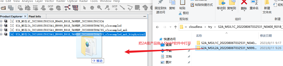
1C级产品生成云掩膜后再批量进行sen2cor大气校正
然后把校正后的2A级产品用SNAP打开

1.2 导入2A级产品

在这里插入图片描述
你应该知道吧，先重采样到你先要的分辨率，这里我们选择10m.

1.3导入我们在第1步生成的云掩膜文件

这时候就要进行我们的掩膜操作了（有什么疑问的去看官方文档，点一下“帮助”认真读一下）
在这里插入图片描述
找到vector Data文件夹，选中之后点击上方菜单栏Vector-import-shp

记得这里选否不然每个多边形都生成一个文件

可以看导在Vector Data下面和Masks下面多了一个mask
双击打开可以看到它的属性值，1代表有效像素，0代表无效像素，我们需要抠掉的像素
在这里插入图片描述

这里最好先重采样到10m，我找了一景重采样之后的影像来做演示
看看效果，mask是否完全覆盖了云

然后进行掩膜操作，说白了就是把有云的地方抠掉，然后再进行后续的镶嵌操作补上来，云多真没办法，哎！误差大。

1.4.SNAP掩膜操作

在这里插入图片描述
输入输出参数，选好路径即可

处理参数选择使用矢量掩膜，拉到最后选择我们之前用Python生成的那个shp文件

选择所有波段和下图这四个波段

波段那里全选
。点击run运行即可。
可以看到掩膜之后相当于把云抠掉了
在这里插入图片描述

然后再选取同一传感器，同一地点，相近时间的影像在SNAP软件中做同样的处理
然后把他们镶嵌在一起
在这里插入图片描述
注意是选择dim文件，对话框里面有三个选项卡，I/O Parameters(输入输出参数)，Map Projection Definition
(定义投影)和Variables&Coniditions(变量和条件)。首先我们在输入输出参数选项卡中指定输入的影像，点击下面箭头指向的"加号”即可选择所需影像文件。在本选项卡内还需要对Nme(文件名)、文件输出类型和目录进行设置。
在这里插入图片描述

在这里插入图片描述

运行完毕！

1.5采用gdal计算各类植被指数

Sentinel-2 影像文件名 s.tif，然后使用以下命令将指数计算转换为 GDAL python本地计算
安装gdal库，安装gdal库建议采用本地安装，去下载whl文件，然后转到放置whl文件的目录下，pip install 即可
进入安装好gdal库的虚拟环境，然后将gdal_calc.py下载地址和s.tif文件放在同一个文件夹下。
1.点击开始界面，打开anaconda promopt
在这里插入图片描述
进入S2.tiff所在的文件夹路径

E:
cd E:\2023wanzhou

在这里插入图片描述

运行run.bat

运行之后会在文件夹内生成植被指数。

run.bat的内容如下：S2.tif代表我们要计算植被指数的影像，band=4代表S.tif的B4波段，rvi.tif表示输出影像的文件名，执行的波段运算是B/A也就是B8/B4也就是NIR/RED=RVI

#1.RVI：
python gdal_calc.py -A S2.tif --A_band=4 -B S2.tif --B_band=8 --outfile=rvi.tif --calc="(B/A)" --NoDataValue=0

#2.IPVI：
python gdal_calc.py -A S2.tif --A_band=4 -B S2.tif --B_band=8 --outfile=ipvi.tif --calc="(B/(A+B))" --NoDataValue=0

#3.PVI：
python gdal_calc.py -A S2.tif --A_band=4 -B S2.tif --B_band=8 --outfile=pvi.tif --calc="(sin(pi/4)*B)-(cos(pi/4)*A)" --NoDataValue=0

#4.IRECI：
python gdal_calc.py -A S2.tif --A_band=4 -B S2.tif --B_band=8 --outfile=ireci.tif --calc="((B-A)/(B+A))" --NoDataValue=0

#5.S2AVI：
python gdal_calc.py -A S2.tif --A_band=4 -B S2.tif --B_band=8 --outfile=savi.tif --calc="((B-A)/(B+A+0.5))*(1+0.5)" --NoDataValue=0

#6.ARVI：
python gdal_calc.py -A S2.tif -B S2.tif -C S2.tif --A_band=4 --B_band=8 --C_band=2 --outfile=arvi_wanzhou.tif --calc="((B-(2*A-C))/(B+(2*A-C)))" --NoDataValue=0

#7.PS2S2Ra：
python gdal_calc.py -A S2.tif --A_band=4 -B S2.tif --B_band=7 --outfile=pS2S2ra.tif --calc="(B/A)" --NoDataValue=0

#8.MTCI：
python gdal_calc.py -A S2.tif --A_band=4 -B S2.tif --B_band=5 -C S2.tif --C_band=6 --outfile=mtci.tif --calc="((B-C)/(C-A-0.01))" --NoDataValue=0

#9.MCARI：
python gdal_calc.py -A S2.tif --A_band=4 -B S2.tif --B_band=5 -C S2.tif --C_band=3 --outfile=mcari.tif --calc="((B-A)-(0.2*(B-C)))*(B-A)" --NoDataValue=0

#10.REIP：
python gdal_calc.py -A S2.tif --A_band=4 -B S2.tif --B_band=5 -C S2.tif --C_band=6 -D S2.tif --D_band=7 --outfile=reip.tif --calc="(700)+(40*((B+D)/2-A)/(C-A))" --NoDataValue=0

#11.NDVI78a (NIR2 – RE3)/ (NIR2 + RE3)
python gdal_calc.py -A S2.tif --A_band=8 -B S2.tif --B_band=7 --outfile=ndvi78a.tif --calc="(A-B)/(A+B)" --NoDataValue=0

#12.NDVI67 (RE3- RE2)/ (RE3+ RE2)
python gdal_calc.py -A S2.tif --A_band=7 -B S2.tif --B_band=6 --outfile=ndvi67.tif --calc="(A-B)/(A+B)" --NoDataValue=0

#13.NDVI58a (NIR2- RE1)/ (NIR2 + RE1)
python gdal_calc.py -A S2.tif --A_band=8 -B S2.tif --B_band=5 --outfile=ndvi58a.tif --calc="(A-B)/(A+B)" --NoDataValue=0

#14.NDVI56 (RE2- RE1)/ (RE2+ RE1)
python gdal_calc.py -A S2.tif --A_band=6 -B S2.tif --B_band=5 --outfile=ndvi56.tif --calc="(A-B)/(A+B)" --NoDataValue=0

#15.NDVI57 (RE3- RE1)/ (RE3+ RE1)
python gdal_calc.py -A S2.tif --A_band=7 -B S2.tif --B_band=5 --outfile=ndvi57.tif --calc="(A-B)/(A+B)" --NoDataValue=0

#16.NDVI68a (NIR2 - RE2)/ (NIR2 + RE2)
python gdal_calc.py -A S2.tif --A_band=8 -B S2.tif --B_band=6 --outfile=ndvi68a.tif --calc="(A-B)/(A+B)" --NoDataValue=0

#17.NDVI48 (NIR - R)/ (NIR + R)
python gdal_calc.py -A S2.tif --A_band=8 -B S2.tif --B_band=4 --outfile=ndvi48.tif --calc="(A-B)/(A+B)" --NoDataValue=0

1.6 纹理特征参数提取

采用envi软件
有研究表明，遥感数据的纹理信息能够增强原始影像亮度的空间信息辨识度，提升地表参数的反演精度。本研究采用灰度共生矩阵( gray level co-occurrence matrix，GLCM) 提取纹理特征信息，究纹理窗口大小设置为 3×3，获取8类纹理特征值。
灰度共生矩阵提取纹理特征信息可参考
在这里插入图片描述
处理完后可将纹理信息提取出来，可通过APP store 中的Split to Multiple Single-Band Files 工具进行直接拆分
Sentinel-2中10个波段每个波段的纹理信息共80个

二.哨兵1号获取/处理/提取数据

哨兵1号数据在欧空局中下载，然后采用SNAP软件对其进行一系列处理
可参考链接
多幅影像建议镶嵌完-计算纹理信息-波段拆分-处理后记得把坐标系和投影转成和哨兵2号一样

2.1 纹理特征参数提取

同1.3
基于 VH 和VV 极化影像提取纹理特征信息，获取 8X2=16 个纹理特征
在这里插入图片描述

三、DEM数据

3.1 数据下载

可参考这篇文章进行数据下载

3.2 数据处理

一定要注意呀！
获取的数据是30m分辨率的，哨兵数据是10米分辨率，在arcGis中搜索resample 需要将DEM重采样到10米分辨率。
然后在ArcGis中搜索坡度和坡向这两个工具，分别计算这两变量。

四、样本生物量计算

代码如下，d代表胸径，h代表树高
查找优势树种对应的异速生长方程写上就行


import pandas as pd
# 读取 CSV 文件
df = pd.read_csv('E:\Sentinel12\yangben\yangben.csv', encoding='gbk')
# 定义优势树种类型及对应的
tree_types = {
    '柏木': lambda d, h: 0.12703 * (d ** 2 * h )** 0.79775,
    '刺槐': lambda d, h: ( 0.05527 * (d ** 2 * h )** 0.8576) + (  0.02425* (d ** 2 * h )** 0.7908) +( 0.0545 * (d ** 2 * h )** 0.4574),
     #http://www.xbhp.cn/news/11502.html
    '栎类': lambda d, h:0.16625 * ( d ** 2 * h ) ** 0.7821,
    '柳杉': lambda d, h:( 0.2716 * ( d ** 2 * h ) ** 0.7379 ) + ( 0.0326 * ( d ** 2 * h ) ** 0.8472 ) + ( 0.0250 * ( d ** 2 * h ) ** 1.1778 ) + ( 0.0379 * ( d ** 2 * h ) ** 0.7328 ),
    '马尾松': lambda d, h: 0.0973 * (d ** 2 * h )** 0.8285,
    '其他硬阔': lambda d, h:( 0.0125 * (d ** 2 * h )**1.05 ) + (  0.000933* (d ** 2 * h )**1.23 ) +( 0.000394 * (d ** 2 * h )** 1.20),
    '杉木': lambda d, h: ( 0.00849 * (d ** 2 * h) ** 1.107230) + ( 0.00175 * (d ** 2 * h )** 1.091916) + 0.00071 * d **3.88664 ,
    '湿地松': lambda d, h: 0.01016* (d ** 2 * h )**1.098,
    '香樟': lambda d, h:( 0.05560 * (d ** 2 * h )** 0.850193) + ( 0.00665 * (d ** 2 * h )** 1.051841) +( 0.05987 * (d ** 2 * h )** 0.574327)+( 0.01476 * (d ** 2 * h )** 0.808395) ,
    '油桐': lambda d, h: ( 0.086217 *d ** 2.00297)+ ( 0.072497 *d ** 2.011502)+( 0.035183 *d ** 1.63929),
    '杨树': lambda d, h: ( 0.03 * (d ** 2 * h )** 0.8734) + ( 0.0174 * (d ** 2 * h )** 0.8574) +( 0.4562 * (d ** 2 * h )** 0.3193)+( 0.0028 * (d ** 2 * h )**0.9675 ) ,
}

# 遍历样本并计算地上生物量```python
for i, row in df.iterrows():
    tree_type = row['优势树']
    if tree_type in tree_types:
        d = row['平均胸径']
        h = row['林分平均树高']
        biomass = tree_types[tree_type](d, h)
        df.at[i, '生物量'] = biomass

# 将计算后的地上生物量写入 CSV 文件
df.to_csv('E:\Sentinel12\yangben\yangben_processed.csv', index=False)

五、样本变量选取

将样本导入arcgis,设置好投影信息，在ArcGis中找到多值提取至点工具。
参考这篇文章

六、随机森林建模

参考1
参考2
可以用SPSS进行相关性分析，可参考,选择相关性比较大的变量进行建模
随机森林代码如下：

6.1导入库与变量准备

提前将excel转为csv格式，用用记事本转化下编码防止程序读取时出现乱码，另存为右下角编码改为UTF-8。
在这里插入图片描述

记得安装sklearn包
命令行如下：

pip install scikit-learn

本文中设计到的所有python代码均在jupyter notebook中运行

import pandas as pd
import numpy as np
from matplotlib import pyplot as plt
from sklearn.ensemble import RandomForestRegressor
from sklearn.model_selection import train_test_split
from sklearn.metrics import mean_squared_error, r2_score
from pyswarm import pso
import rasterio #缺少库时，在jupyter中使用!pip install rasterio命令，加!相当于在cmd窗口运行安装 
# import pydot
import numpy as np
import pandas as pd
import scipy.stats as stats
from pprint import pprint
from sklearn import metrics
from sklearn.model_selection import GridSearchCV
from sklearn.model_selection import RandomizedSearchCV
from joblib import dump
# 读取Excel表格数据
data = pd.read_csv(r'E:\Sentinel12\yangben\建模\jianmo.csv' )
y = data.iloc[:, 0].values  # 生物量
X = data.iloc[:, 1:].values  # 指标变量
df = pd.DataFrame(data)
random_seed=44
random_forest_seed=np.random.randint(low=1,high=230)
# 分割数据集为训练集和测试集
X_train, X_test, y_train, y_test = train_test_split(X, y, test_size=0.3, random_state=42)

运行完这个代码块，可以打印一下，看看变量长什么样。这里可以看到，选取的变量一共有5个，值分别为1.11691217e+01, 4.37000000e+02, 1.31032691e+00, 7.31299972e-01, 1.13057424e-01 可以打开样本表看看，这五个变量对应的值是否正确。
在这里插入图片描述

6.2 选取参数

决策树个数n_estimators

决策树最大深度max_depth，

最小分离样本数（即拆分决策树节点所需的最小样本数） min_samples_split，

最小叶子节点样本数（即一个叶节点所需包含的最小样本数）min_samples_leaf，

最大分离特征数（即寻找最佳节点分割时要考虑的特征变量数量）max_features

# Search optimal hyperparameter
#对六种超参数划定了一个范围，然后将其分别存入了一个超参数范围字典random_forest_hp_range
n_estimators_range=[int(x) for x in np.linspace(start=50,stop=3000,num=60)]
max_features_range=['sqrt','log2',None]
max_depth_range=[int(x) for x in np.linspace(10,500,num=50)]
max_depth_range.append(None)
min_samples_split_range=[2,5,10]
min_samples_leaf_range=[1,2,4,8]

random_forest_hp_range={'n_estimators':n_estimators_range,
                        'max_features':max_features_range,
                        'max_depth':max_depth_range,
                        'min_samples_split':min_samples_split_range,
                        'min_samples_leaf':min_samples_leaf_range
                        }
random_forest_model_test_base=RandomForestRegressor()
random_forest_model_test_random=RandomizedSearchCV(estimator=random_forest_model_test_base,
                                                   param_distributions=random_forest_hp_range,
                                                   n_iter=200,
                                                   n_jobs=-1,
                                                   cv=3,
                                                   verbose=1,
                                                   random_state=random_forest_seed
                                                   )
random_forest_model_test_random.fit(X_train,y_train)

best_hp_now=random_forest_model_test_random.best_params_
# Build RF regression model with optimal hyperparameters
random_forest_model_final=random_forest_model_test_random.best_estimator_
print(best_hp_now)

可以看到打印结果
在这里插入图片描述

6.3 误差分布直方图

如果直方图呈现正态分布或者近似正态分布，说明模型的预测误差分布比较均匀，预测性能较好。如果直方图呈现偏斜或者非正态分布，说明模型在某些情况下的预测误差较大，预测性能可能需要进一步改进。

# Predict test set data
random_forest_predict=random_forest_model_test_random.predict(X_test)
random_forest_error=random_forest_predict-y_test
    
plt.figure(1)
plt.clf()
plt.hist(random_forest_error)
plt.xlabel('Prediction Error')
plt.ylabel('Count')
plt.grid(False)
plt.show()

在这里插入图片描述

6.4 变量重要性可视化展示

# 计算特征重要性
random_forest_importance = list(random_forest_model_final.feature_importances_)
random_forest_feature_importance = [(feature, round(importance, 8)) 
                                    for feature, importance in zip(df.columns[4:], random_forest_importance)]
random_forest_feature_importance = sorted(random_forest_feature_importance, key=lambda x:x[1], reverse=True)

# 将特征重要性转换为Pyecharts所需的格式
x_data = [item[0] for item in random_forest_feature_importance]
y_data = [item[1] for item in random_forest_feature_importance]

# 绘制柱状图
bar = (
    Bar()
    .add_xaxis(x_data)
    .add_yaxis("", y_data)
    .reversal_axis()
    .set_series_opts(label_opts=opts.LabelOpts(position="right"))
    .set_global_opts(
        title_opts=opts.TitleOpts(title="Variable Importances"),
        xaxis_opts=opts.AxisOpts(name="Importance",axislabel_opts=opts.LabelOpts(rotate=-45, font_size=10)),
        yaxis_opts=opts.AxisOpts(name_gap=30, axisline_opts=opts.AxisLineOpts(is_show=False)),
        tooltip_opts=opts.TooltipOpts(trigger="axis", axis_pointer_type="shadow")
    )
)

bar.render_notebook()

在这里插入图片描述

6.5 对精度进行验证

这里可输出相关的精度值

# Verify the accuracy
random_forest_pearson_r=stats.pearsonr(y_test,random_forest_predict)
random_forest_R2=metrics.r2_score(y_test,random_forest_predict)
random_forest_RMSE=metrics.mean_squared_error(y_test,random_forest_predict)**0.5
print('Pearson correlation coefficient = {0}、R2 = {1} and RMSE = {2}.'.format(random_forest_pearson_r[0],random_forest_R2,random_forest_RMSE))

6.6 预测生物量

注意几个tif数据的nodata值不一样，最好全部都将nodata值设为0，最后得到的biomass图像按照掩膜提取，nodata就变回来啦

import numpy as np
import rasterio
from tqdm import tqdm

# 读取五个栅格指标变量数据并整合为一个矩阵
with rasterio.open(r'E:\Sentinel12\yangben\建模\result\nodata\podu.tif') as src:
    data1 = src.read(1)
    meta = src.meta
with rasterio.open(r'E:\Sentinel12\yangben\建模\result\nodata\dem.tif') as src:
    data2 = src.read(1)
with rasterio.open(r'E:\Sentinel12\yangben\建模\result\nodata\lai.tif') as src:
    data3 = src.read(1)
with rasterio.open(r'E:\Sentinel12\yangben\建模\result\nodata\ndvi.tif') as src:
    data4 = src.read(1)
with rasterio.open(r'E:\Sentinel12\yangben\建模\result\nodata\pvi.tif') as src:
    data5 = src.read(1)

X = np.stack((data1, data2, data3, data4, data5), axis=-1)

# 清洗输入数据
X_2d = X.reshape(-1, X.shape[-1])
# 检查数据中是否存在 NaN 值
print(np.isnan(X_2d).any())  # True

# 将 nodata 值替换为0
X_2d[np.isnan(X_2d)] = 0

# 使用已经训练好的随机森林模型对整合后的栅格指标变量数据进行生物量的预测
y_pred = []
for i in tqdm(range(0, X_2d.shape[0], 10000)):
    y_pred_chunk = random_forest_model_test_random.predict(X_2d[i:i+10000])
    y_pred.append(y_pred_chunk)
y_pred = np.concatenate(y_pred)

# 将预测结果保存为一个新的栅格数据
with rasterio.open(r'E:\Sentinel12\yangben\建模\result\biomass_v5.tif', 'w', **meta) as dst:
    dst.write(y_pred.reshape(X.shape[:-1]), 1)
print("预测结束")

运行之后会在下面出现进度条，进度条走完了就代码预测完了
在这里插入图片描述

七、生物量制图

7.1. 将得到的biomass.tif文件按掩膜提取

 掩膜文件选择用于预测的tif文件，目的是将nodata值还原回来。

7.2. 提取森林掩膜区域

[参考链接](https://www.bilibili.com/video/BV1qv4y1A75B?p=10&vd_source=ddb0eb9d8fde0d0629fc9f25dc6915e5)

这里需要全球土地覆盖10米的更精细分辨率观测和监测（FROM-GLC10）数据。
我们在GEE平台上下载研究区的GLC10图，参考链接

在 Google Earth Engine Code Editor 中搜索“ESA Global Land Cover 10m v2.0.0”并加载该数据集。

var glc = ee.Image('ESA/GLOBCOVER_L4_200901_200912_V2_3');

定义您感兴趣的区域。
这里的table需要先将shp文件上传到平台，再点那个小箭头导入

这里就会有table出现

var geometry = table;

使用 Image.clip() 函数将图像裁剪为您感兴趣的区域。

var clipped = glc.clip(geometry);

使用 Export.image.toDrive() 函数导出图像。以下代码将图像导出到您的 Google Drive 中。

Export.image.toDrive({
  image: clipped,
  description: 'GLC',
  folder: 'my_folder',
  scale: 10,
  region: geometry
});

其中，description 是导出图像的名称，folder 是导出图像的文件夹，scale 是导出图像的分辨率，region 是导出图像的区域。

点击“Run”按钮运行代码。代码运行完成后，您可以在 Google Drive 中找到导出的图像文件。

20序号代表森林，按属性提取，可以把森林提取出来，按属性提取工具。

重采样到10m,定义投影

将生物量.tif按照掩膜tif掩膜即可得到森林区域的生物量。

八. 需要注意的点

每个栅格变量数据一定要保持行数和列数一致，这不仅是为了”多值提取至点“等一一对应，更是为了最后估算生物量的时候生成二维矩阵输入模型，保证输入数据的维度一致。
第一步的前提是第二部，投影！投影！投影!重要的事情说三遍，一定要在相同坐标系下面
注意nodata值的处理，最好所有的影像nodata设置为0,这样最后输入模型中可以减少计算量。

参考：https://blog.csdn.net/weixin_45276304/article/details/132214597?spm=1001.2014.3001.5502
https://blog.csdn.net/weixin_45276304/article/details/132037984?spm=1001.2014.3001.5502
https://blog.csdn.net/weixin_45276304/article/details/132320219?spm=1001.2014.3001.5502

2301_79407279

关注

2
点赞
踩
18

收藏

觉得还不错? 一键收藏
1
评论
森林生物量估算

run.bat的内容如下：S2.tif代表我们要计算植被指数的影像，band=4代表S.tif的B4波段，rvi.tif表示输出影像的文件名，执行的波段运算是B/A也就是B8/B4也就是NIR/RED=RVI。运行完之后，我们会得到一个tif文件，因为我们只需要云掩膜也就是保留0和1的像元（纯净的陆地像素与纯净的水像素），其他和云相关的像元删掉，也就是将云所在的像素去掉。然后进行掩膜操作，说白了就是把有云的地方抠掉，然后再进行后续的镶嵌操作补上来，云多真没办法，哎！
复制链接

扫一扫