


目录
说明:
1.网上 Pytorch 自然语言处理中情感分析的相关代码使用的大多是同一个数据集,且这些代码都具有较高的相似程度和较难的理解程度,而本文提供了相对简洁易懂的 txt 版本,供大家进行参考。另一个类似的自然语言处理中文本多分类的 csv 版本的代码会在后续的文章中发布。这两个版本可以提供不同数据集形式的基础代码框架,为大家的学习节省一定的时间
2.代码运行环境:google colab(GPU模式)
3.数据集:本项目使用的数据集是经过处理的以 txt 文件形式储存的的影评数据集,包括影评内容和影评标签两个 txt 文件。因此,以下代码均是以 txt 文件为基础进行处理的。
一、数据集 txt 文件导入
import numpy as np
import pandas as pd
from google.colab import drive

drive.mount('/content/drive')
txt_text_path = '/content/drive/MyDrive/film_comment_text.txt'
txt_label_path = '/content/drive/MyDrive/film_comment_label.txt'

with open(txt_text_path, 'r', encoding='utf-16') as f:
    text = f.read()

with open(txt_label_path, 'r', encoding='utf-16') as f:
    label = f.read()

len(text)

# 运行结果,查看一下影评内容的总体长度为多少
59235849
二、影评及标签预处理
2.1 删除影评标点符号
from string import punctuation
clean_text = ''.join([char for char in text if char not in punctuation])
len(clean_text)

# 运行结果,可以看到相比之前影评内容的总体长度有所减少
56662182
2.2 将影评及对应标签按照换行符分隔
clean_text = clean_text.split('\n')
print(len(clean_text)

label = label.split('\n')
print(len(label))

# 运行结果,需要注意的是,经过处理影评内容和对应的标签行数一定要是相同的,不然会出现数据行数不匹配的现象
45001
45001
2.3 影评内容清洗
import re

# 定义清洗文本的函数
def remove(text):
    # 使用正则表达式替换非英文字母字符为空
    text = text.lower()
    return re.sub(r'[^A-Za-z\s]+', '', text)

# 对列表中的每个字符串应用清洗函数,用以下的代码写循环运行效率比较高
clean_text = [remove(text) for text in clean_text]

# 可以选择输出第一个影评内容进行查看
# clean_text[0]
三、创建词汇表与字典
3.1 创建词汇表
def vocab_build(text_list):
	# 定义一个集合,来存储不同的单词
    unique_words = set()
    for text in text_list:
        # 以空格分隔单词
        words = text.split()
        # update 方法用于将新的单词添加到 unique_words 集合中
        unique_words.update(words)
    return unique_words

# 将之前经过处理的 clean_text 传入函数
vocab = vocab_build(clean_text)
vocab = list(vocab)
len(vocab)

# 运行结果,可以看到创建的词汇表中不同的单词个数
165857
3.2 创建字典:单词 → 索引
# 创建字典格式:(整数: 单词)
int_word_dict = dict(enumerate(vocab, 1))
# 转换字典格式:(单词: 整数)
word_int_dict = {w:int(i) for i, w in int_word_dict.items()}
3.3 将影评标签进行 0,1 的转换
# 0 表示 Negative,1 表示 Positive
label_int = np.array([0 if x == 'Negative' else 1 for x in label])
len(label_int)

# 运行结果,可以看到与之前 label 的行数相同
45001
四、删除过长影评与单词映射
4.1 删除过长的影评
from collections import Counter

# 定义返回符合删除条件的评论所在行索引的函数
def delete(text_list):
    # 查看数据集中每个影评里单词的数量,并存放到一个列表里
    sentence_length = [len(sentence.split()) for sentence in text_list]
    # 查找长度在 900 以上的影评的索引
    text_index = [i for i, length in enumerate(sentence_length) if length > 900]
    return text_index

# 获取满足删除条件的行索引
index_to_drop = delete(clean_text)
# 查看需要删除多少行的影评内容和对应标签
print(len(index_to_drop))

# 使用了 np.delete() 函数,用于从 clean_text 中删除指定索引的行的影评内容和对应标签
new_text = np.delete(clean_text, index_to_drop)
print(len(new_text))
new_label = np.delete(label_int, index_to_drop)
print(len(new_label))

# 运行结果,可以看到 new_text 与 new_label 的行数依然相同
452
44549
44549
4.2 将单词映射为数字
text_to_int_list = []

# 读取 clean_text 列表中的每条影评
for sentence in new_text:
    sample = list()
    # 根据空格切分 sentence,这样就能读取到每一个单词
    for word in sentence.split():
    	# 将影评中的每个单词转变成其在词汇表中的索引值
        int_value = word_int_dict[word]
        sample.append(int_value)
    text_to_int_list.append(sample)

# 查看第一条影评转换的数字索引列表
# text_to_int_list[0]
五、影评长度截断
# 设定每条评论的固定长度是 500 个单词,单词数量不足的评论用 0 填充,超过的直接截断
# 定义评论长度固定函数
def reset_text(text, seq_len):
    # 初始化一个全为 0 的矩阵,形状为 (评论数量 * 评论长度)
    text_dataset = np.zeros((len(text), seq_len))
    # 读取每一条评论的索引和内容
    for index, sentence in enumerate(text):
        # 如果评论长度小于 500,用 0 进行填充
        if len(sentence) < seq_len:
            text_dataset[index, :len(sentence)] = sentence
        else:
            # 如果评论长度大于 500,截断
            text_dataset[index, :] = sentence[:seq_len]
    return text_dataset

dataset = reset_text(text_to_int_list, seq_len=500)
六、Pytorch 数据类型转换与数据集划分
6.1 数据类型转换(tensor)
import torch

# 查看 dataset 和 label_int 的数据类型
print(type(dataset))
print(type(label_int))

# 将 dataset 和 label_int 转换为 pytorch 中的 tensor 形式
dataset_tensor = torch.from_numpy(dataset)
label_tensor = torch.from_numpy(new_label)

print(dataset_tensor.shape)
print(label_tensor.shape)

# 运行结果
<class 'numpy.ndarray'>
<class 'numpy.ndarray'>
torch.Size([44549, 500])
torch.Size([44549])
6.2 数据集划分和获取
# 总样本数
all_samples = len(dataset_tensor)
print(f'总样本数:{all_samples}')

# 训练样本数,取总样本数的 80%
train_size = int(all_samples * 0.8)
print(f'训练样本数:{train_size}')

rest_size = all_samples - train_size

# 测试样本数
test_size = int(rest_size)
print(f'测试样本数:{test_size}')

# 运行结果
总样本数:44549
训练样本数:35639
测试样本数:8910
# 获取 train,test 数据集的样本
train_text = dataset_tensor[:train_size]
train_label = label_tensor[:train_size]
print(f'训练集影评大小:{train_text.shape}')
print(f'训练集影评标签大小:{train_label.shape}')

rest_samples = dataset_tensor[train_size:]
rest_labels = label_tensor[train_size:]

test_text = rest_samples[:test_size]
test_label = rest_labels[:train_size]
print(f'测试集影评大小:{test_text.shape}')
print(f'测试集影评标签大小:{test_label.shape}')

# 运行结果
训练集影评大小:torch.Size([35639, 500])
训练集影评标签大小:torch.Size([35639])
测试集影评大小:torch.Size([8910, 500])
测试集影评标签大小:torch.Size([8910]
七、Pytorch 构建 Dataloader 加载并按批处理数据
from torch.utils.data import TensorDataset, DataLoader
from torchtext.data.functional import to_map_style_dataset

# 对数据进行封装 (评论,标签)
train_dataset = TensorDataset(train_text, train_label)
test_dataset = TensorDataset(test_text, test_label)

batch_size = 64
# Dataloader在每一轮迭代结束后,重新生成索引并将其传入到 to_map_style_dataset 中,就能返回一个个样本
# shuffle=True 表示打乱样本顺序
# collate_fn 可以对 Dataloader 生成的 mini-batch 进行后处理
# pin_memory=True 表示使用 GPU
# drop_last=True 表示若最后数据量不足 64 个,则将其全部舍弃
train_loader = DataLoader(to_map_style_dataset(train_dataset), batch_size=batch_size, pin_memory=True, shuffle=True, drop_last=True)
test_loader = DataLoader(to_map_style_dataset(test_dataset), batch_size=batch_size, pin_memory=True, shuffle=False, drop_last=True)
# 获取 train 中的一批数据
data, label = next(iter(train_loader))
print(data.shape)
print(label.shape)

# 运行结果
torch.Size([64, 500])
torch.Size([64])
# 将设备转换成 colab 中的 GPU 模式
device = torch.device("cuda:0" if torch.cuda.is_available() else "cpu")
八、LSTM 模型定义
batch_size = 64
# 每个评论列表的大小
seqLen = 500
# 词汇表的大小 + 1
input_size = len(vocab) + 1
# 总共有2个类别,但是输出维度可以设置成 1
output_size = 1
#词嵌入层维度
embedding_size = 300
# 隐藏层维度
hidden_size = 128
# LSTM 层数
num_layers = 1
# epoch 次数
num_epoch = 20

class Sentiment(torch.nn.Module):
    def __init__(self, input_size, embedding_size, hidden_size, output_size, num_layers, dropout=0.5):
        super(Sentiment, self).__init__()
        self.hidden_size = hidden_size
        self.output_size = output_size
        self.num_layers = num_layers
        # 将输入的文本进行词嵌入表示的操作,即将 input_size 转变为 embedding_size
        self.embedding = torch.nn.Embedding(input_size, embedding_size)
        # LSTM 的输入维度就是 embedding_size,即 300。batch_first=True 表示将 batch_size 设置成第一个维度
        self.lstm = torch.nn.LSTM(embedding_size, hidden_size, num_layers, batch_first=True)
        self.dropout = torch.nn.Dropout(dropout)
        # 全连接层,其中 output_size 就是类别数量,即 1
        self.linear = torch.nn.Linear(hidden_size, output_size)
        self.sigmoid = torch.nn.Sigmoid()

    def forward(self, x):
        '''
        x original shape: (seqLen, batch_size, input_size)
        x transform shape (batch_first=True) : (batch_size, seqLen, input_size)
        batch_size:一组数据有多少个,即 64
        seqLen:每个影评列表中有多少个单词,即 500
        input_size:每个影评列表中,每个数字代表的单词的数量,即词汇表大小 + 1
        '''
        batch_size = x.size(0)
        # 将输入的影评转换为长整型,形状为 (batch_size, seqLen, input_size)
        x = x.long()
        # 1. 初始化隐藏层中的隐藏状态 h0 (用于传递序列中前一个时间点的信息到下一个时间点),同时将其转移到与输入影评相同的设备上 (即GPU)
        # 2. h0 的形状为 (num_layers, batch_size, hidden_size)
        h0 = torch.zeros(self.num_layers, batch_size, self.hidden_size).to(x.device)
        # 1. 初始化隐藏层中的单元状态 c0 (用于在网络中长期传递信息),同时将其转移到与输入影评相同的设备上 (即GPU)
        # 2. c0 的形状为 (num_layers, batch_size, hidden_size)
        c0 = torch.zeros(self.num_layers, batch_size, self.hidden_size).to(x.device)
        # 输出 x 的形状为 (batch_size, seqLen, embedding_size)
        x = self.embedding(x)
        # 1. 输出 output 的形状为 (batch_size, seqLen, hidden_size)
        # 2. 输出 hn 的形状为 (num_layers, batch_size, hidden_size)
        # 3. 输出 cn 的形状为 (num_layers, batch_size, hidden_size)
        output, (hn, cn) = self.lstm(x, (h0, c0))
        # 1. 选择最后一个时间步的输出
        # 2. 输入 output 的形状变为 (batch_size, hidden_size)
        # 3. 输出 output 的形状变为 (batch_size, output_size)
        output = self.linear(output[:, -1])
        # 输出 output 的形状为 (batch_size, output_size),表示每个序列属于目标类别的概率
        output = self.sigmoid(output)
        return output

model = Sentiment(input_size, embedding_size, hidden_size, output_size, num_layers, dropout=0.5)
model.to(device)
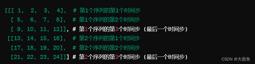
output[:, -1] 代码解释:
假设我们有一个小批量的输出 output,其形状为(2, 3, 4),这表示我们有 2 个序列,每个序列有 3 个时间步,每个时间步的输出是一个 4 维的向量,如下图所示:
当执行 output[:, -1] 时,我们选择每个序列的最后一个时间步的输出,即每个序列的第 3 个时间步。这样,我们得到的结果如下图所示:
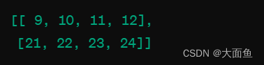
在我们这个例子中,output 的形状是 (64, 500, 128),这表示对于 64 个影评,每个影评有 500 个时间步(也即每个影评列表中统一的单词数),每个时间步的输出是一个 128 维的向量。这个输出代表了 LSTM 网络在每个时间步对每个影评的处理结果。
当执行 output[:, -1] 这个操作时,我们是在选择每个影评的最后一个时间步的输出。这意味着从每个影评中,我们只取出该序列经过 LSTM 处理后的最终状态,忽略之前所有时间步的输出。因此,对于 64 个影评,每个影评最终只对应一个 128 维的向量,这个向量概括了整个影评的信息。
import torch.optim as optim

# 定义交叉熵损失函数
criterion = torch.nn.BCELoss()
# 定义 Adam 优化器,weight_decay 表示 L2 正则化,为了防止过拟合的情况发生
optimizer = optim.Adam(model.parameters(), lr=0.01, weight_decay=1e-5)
九、测试与训练函数定义
def test(model, data_loader, device, criterion):
    model.eval()
    test_loss = 0
    test_correct = 0
    total = 0

	# 测试函数无需梯度计算
    with torch.no_grad():
        for data, target in data_loader:
        	# 将 batch 中的每一对样本数据都传到 GPU 设备上
            data, target = data.to(device), target.to(device)
            # 获得输出结果
            output = model(data)
            # 1. 计算损失
            # 2. output.squeeze() 的目的是移除 output 中大小为1的维度
            # 3. 如果 output 的形状是 (N, 1),那么 squeeze() 会将其形状改为(N,)
            loss = criterion(output.squeeze(), target.float())
            # 损失累加
            test_loss += loss.item()

			# 1. 如果 output 的值大于 0.5,则 pred 为 True,否则为 False
			# 2. 例如,output=[0.8, 0.3, 0.6],则 pred=[True, False, True]
            pred = output.squeeze() > 0.5
            # 1. 将 pred 与 target 转换的布尔值作比较
            # 2. 例如,pred=[True, False, True],target=[True, False, False] (target 转换前的值为 [1, 0, 1])
            # 3. 那么就意味着有 2 个样本预测正确了,并累加预测正确的样本数量,即 2
            test_correct += torch.sum(pred == target.bool()).item()
            total += target.size(0)

	# 计算评价损失和平均准确率
    average_loss = test_loss / len(data_loader)
    average_accuracy = test_correct / total * 100
    return average_loss, average_accuracy
def train(model, device, train_loader, test_loader, criterion, optimizer, num_epoch, lambda_l1=0.001):
    for epoch in range(num_epoch):
        model.train()
        train_loss = 0
        train_correct = 0
        total = 0
        for data, target in train_loader:
            data, target = data.to(device), target.to(device)
            optimizer.zero_grad()
            output = model(data)
            loss = criterion(output.squeeze(), target.float())
            loss.backward()
            optimizer.step()

            train_loss += loss.item()
            pred = output.squeeze() > 0.5
            train_correct += torch.sum(pred == target.bool()).item()
            total += target.size(0)

        train_accuracy = train_correct / total * 100

        # 在每个 epoch 中后调用测试模型返回的结果,以计算测试损失和测试准确率
        test_loss, test_accuracy = test(model, test_loader, device, criterion)

        print(f'Epoch: {epoch+1}/{num_epoch} | '
              f'Train Loss: {train_loss / len(train_loader):.5f} | '
              f'Train Accuracy: {train_accuracy:.2f}% | '
              f'Test Loss: {test_loss:.5f} | '
              f'Test Accuracy: {test_accuracy:.2f}%')

train(model, device, train_loader, test_loader, criterion, optimizer, num_epoch)

# 运行结果
Epoch: 1/20 | Train Loss: 0.69537 | Train Accuracy: 50.14% | Test Loss: 0.69366 | Test Accuracy: 49.65%
Epoch: 2/20 | Train Loss: 0.69377 | Train Accuracy: 50.59% | Test Loss: 0.69321 | Test Accuracy: 50.48%
Epoch: 3/20 | Train Loss: 0.69374 | Train Accuracy: 49.88% | Test Loss: 0.69370 | Test Accuracy: 50.19%
Epoch: 4/20 | Train Loss: 0.69370 | Train Accuracy: 49.76% | Test Loss: 0.69315 | Test Accuracy: 50.33%
Epoch: 5/20 | Train Loss: 0.69358 | Train Accuracy: 50.15% | Test Loss: 0.69338 | Test Accuracy: 49.84%
Epoch: 6/20 | Train Loss: 0.69351 | Train Accuracy: 49.92% | Test Loss: 0.69386 | Test Accuracy: 50.09%
Epoch: 7/20 | Train Loss: 0.69342 | Train Accuracy: 49.92% | Test Loss: 0.69377 | Test Accuracy: 50.39%
Epoch: 8/20 | Train Loss: 0.69518 | Train Accuracy: 50.33% | Test Loss: 0.69350 | Test Accuracy: 49.84%
Epoch: 9/20 | Train Loss: 0.69344 | Train Accuracy: 50.19% | Test Loss: 0.69352 | Test Accuracy: 49.84%
Epoch: 10/20 | Train Loss: 0.69248 | Train Accuracy: 50.35% | Test Loss: 0.69600 | Test Accuracy: 50.45%
Epoch: 11/20 | Train Loss: 0.68656 | Train Accuracy: 52.99% | Test Loss: 0.68290 | Test Accuracy: 56.23%
Epoch: 12/20 | Train Loss: 0.65604 | Train Accuracy: 60.72% | Test Loss: 0.67850 | Test Accuracy: 57.99%
Epoch: 13/20 | Train Loss: 0.58610 | Train Accuracy: 68.99% | Test Loss: 0.54426 | Test Accuracy: 73.43%
Epoch: 14/20 | Train Loss: 0.50146 | Train Accuracy: 76.05% | Test Loss: 0.49358 | Test Accuracy: 76.62%
Epoch: 15/20 | Train Loss: 0.40769 | Train Accuracy: 82.04% | Test Loss: 0.43775 | Test Accuracy: 80.68%
Epoch: 16/20 | Train Loss: 0.34408 | Train Accuracy: 85.50% | Test Loss: 0.42319 | Test Accuracy: 81.74%
Epoch: 17/20 | Train Loss: 0.31500 | Train Accuracy: 86.81% | Test Loss: 0.42676 | Test Accuracy: 81.70%
Epoch: 18/20 | Train Loss: 0.30259 | Train Accuracy: 87.81% | Test Loss: 0.40397 | Test Accuracy: 82.53%
Epoch: 19/20 | Train Loss: 0.28809 | Train Accuracy: 88.33% | Test Loss: 0.39623 | Test Accuracy: 83.64%
Epoch: 20/20 | Train Loss: 0.26917 | Train Accuracy: 89.21% | Test Loss: 0.40100 | Test Accuracy: 83.63%
十、影评情感预测模型定义
def predict(model, text, device):
    new_text = ''.join([char for char in text if char not in punctuation])
    # 文本映射成索引
    text_ints = [word_int_dict[word.lower()] for word in new_text.split()]
    # 对齐文本
    new_text_ints = reset_text([text_ints], seq_len=500)
    text_tensor = torch.from_numpy(new_text_ints)
    batch_size = text_tensor.size(0)
    text_tensor = text_tensor.to(device)
    pred = model(text_tensor)
    print(f'Probability: {pred.item()}')
    # 将概率值转换为 0 或 1
    pred = torch.round(pred)
    print(f'Category value: {pred.item()}')
    if pred.data == 1:
        print('Predict: Positive film review')
    else:
        print('Predict: Negative film review')

text = "this movie is so great, I really like it."
predict(model, text, device)

# 运行结果
Probability: 0.8856309652328491
Category value: 1.0
Predict: Positive film review


 876
876


 被折叠的 条评论
为什么被折叠?
被折叠的 条评论
为什么被折叠?
 到【灌水乐园】发言


