python随机森林特征重要性,python随机森林分类模型

大家好，小编来为大家解答以下问题，python随机森林特征重要性，python随机森林分类模型，今天让我们一起来看看吧！

以下内容笔记出自‘跟着迪哥学python数据分析与机器学习实战’，外加个人整理添加，仅供个人复习使用。

---

这里以一个例子切入随机森林的建模，使用随机森林弯沉对天气最高温度的预测

1. 导入数据

import pandas as pd
import matplotlib.pyplot as plt
%matplotlib inline
import warnings
warnings.filterwarnings('ignore')
import os
#os.chdir()

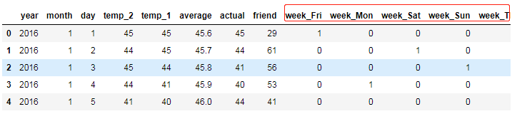
features=pd.read_csv(r'data\temps.csv')
print(features.shape)
features.head(2)

2. 数据探索

2.1 时间数据规范获取

import datetime

years=features['year']
months=features['month']
days=features['day']
#datetime格式
dates=[str(int(year))+'-'+str(int(month))+'-'+str(int(day))
      for year,month,day in zip(years,months,days)]
dates=[datetime.datetime.strptime(date,'%Y-%m-%d') for date in dates]

dates[:5]

[datetime.datetime(2016, 1, 1, 0, 0),
datetime.datetime(2016, 1, 2, 0, 0),
datetime.datetime(2016, 1, 3, 0, 0),
datetime.datetime(2016, 1, 4, 0, 0),
datetime.datetime(2016, 1, 5, 0, 0)]
逻辑是先将原数据中的时间变量组合，转化为时间格式，然后再分割成事件类型的数据python编程代码画爱心。

2.2 时间序列作图

查看最高气温、前天、昨天、friend列的数据值

import seaborn as sns
fig,ax=plt.subplots(nrows=2,ncols=2,figsize=(10,8))
fig.autofmt_xdate(rotation=45)

ax[0,0].plot(dates,features['actual'])
ax[0,1].plot(dates,features['temp_1'])
ax[1,0].plot(dates,features['temp_2'])
ax[1,1].plot(dates,features['friend'])

2.3 哑变量设置

进行one-hot编码

#help(pd.get_dummies)
features=pd.get_dummies(features)
features.head(2)

3. 标签与数据格式转换

import numpy as np
labels = np.array(features['actual']) #转化为数组

features=features.drop('actual',axis=1)
#名字保存下备用
feature_list=list(features.columns)
#转化为合适格式
features=np.array(features)

4. 建模

4.1 训练集与测试集

from sklearn.model_selection import train_test_split
X_train,X_test,y_train,y_test=train_test_split(features,labels,
                                              test_size=0.25,
                                              random_state=42)
print(X_train.shape,X_test.shape)

(261, 14) (87, 14)

4.2 随机森林

from sklearn.ensemble import RandomForestRegressor
rf=RandomForestRegressor(n_estimators=1000,
                        random_state=42)
rf.fit(X_train,y_train)

RandomForestRegressor(bootstrap=True, ccp_alpha=0.0, criterion=‘mse’,
---------------------------------max_depth=None, max_features=‘auto’,
---------------------------------max_leaf_nodes=None,max_samples=None,
---------------------------------min_impurity_decrease=0.0,
---------------------------------min_impurity_split=None, min_samples_leaf=1,
---------------------------------min_samples_split=2, min_weight_fraction_leaf=0.0,
---------------------------------n_estimators=1000, n_jobs=None, oob_score=False,
---------------------------------random_state=42, verbose=0, warm_start=False)

4.3 模型测试

predictions=rf.predict(X_test)
errors=abs(predictions-y_test)
mape=100*(errors/y_test)
print('MAPE',np.mean(mape))
#平均绝对百分误差

MAPE 6.011244187972058

4.4 可视化展示树

from sklearn.tree import export_graphviz
from IPython.display import Image
import pydotplus
import pydot
from sklearn.externals.six import StringIO

#拿到其中的一棵树
tree5=rf.estimators_[5]
tree5

dot_data=tree.export_graphviz(tree5,
                             out_file=None,
                             feature_names=feature_list,
                             class_names='actual',
                             filled=True,
                             impurity=False,
                             rounded=True,
                             special_characters=True)
graph=pydotplus.graph_from_dot_data(dot_data)
graph.get_nodes()[7].set_fillcolor('#FFF2DD')
Image(graph.create_png())

可以看到，树深度太大，减小树深度：

print('depth:',tree5.tree_.max_depth)
#树深度为15，太大，可以减小树深度

rf_small = RandomForestRegressor(n_estimators=10, max_depth = 3,
                                 random_state=42)
rf_small.fit(X_train, y_train)

# 提取一颗树
tree_small = rf_small.estimators_[5]

# 保存
dot_data=tree.export_graphviz(tree_small,
                             out_file=None,
                             feature_names=feature_list,
                             class_names='actual',
                             filled=True,impurity=True,
                             rounded=True,
                             special_characters=True)
graph=pydotplus.graph_from_dot_data(dot_data)
graph.get_nodes()[7].set_fillcolor('#FFF2DD')
Image(graph.create_png())

注意这个例子是回归类型，因此节点分裂的标准是mse！

5. 特征重要性

importances=list(rf.feature_importances_)
#转换格式
feature_importances=[(feature,round(importance,2)) 
                    for feature,importance in zip(feature_list,importances)]

#排序
feature_importances=sorted(feature_importances,   #列表形式数据的排序
                           key=lambda x:x[1],reverse=True)
#对应打印（直接输出也可）
'''[print('Variable:{:20} Importance:{}'.format(*pair))
for pair in feature_importances]'''
feature_importances

[(‘temp_1’, 0.7),
(‘average’, 0.19),
(‘day’, 0.03),
(‘temp_2’, 0.02),
(‘friend’, 0.02),
(‘month’, 0.01),
(‘year’, 0.0),
(‘week_Fri’, 0.0),
(‘week_Mon’, 0.0),
(‘week_Sat’, 0.0),
(‘week_Sun’, 0.0),
(‘week_Thurs’, 0.0),
(‘week_Tues’, 0.0),
(‘week_Wed’, 0.0)]

#作图
importances=list(rf.feature_importances_)
x_values=list(range(len(importances)))

plt.figure(figsize=(8,5))
plt.bar(x_values,importances,orientation='vertical')
#x轴名字
plt.xticks(x_values,feature_list,rotation='vertical')

plt.ylabel('Impor')
plt.xlabel('Var')
plt.title('Var Impor')

6 用重要特征建模试试

rf_most_impor=RandomForestRegressor(n_estimators=1000,
                                   random_state=42)
#重要特征
important_indices=[feature_list.index('temp_1'),
                  feature_list.index('average')]
train_impor=X_train[:,important_indices]  
#train_features是np.array格式数据，可以直接选列
#而数据框需要.iloc
test_impor=X_test[:,important_indices]

#训练模型
rf_most_impor.fit(train_impor,y_train)
#结果
predictions=rf_most_impor.predict(test_impor)
errors=abs(predictions-y_test)
mape=np.mean(100*(errors/y_test))
print('mape',mape)

mape 6.229055723613811

6.1 预测值与真实值关系

#创建一个表格存储日期和对应的标签数值
ture_data=pd.DataFrame(data={'date':dates,'actual':labels})

#同理，创建表格存储预测值
months=X_test[:,feature_list.index('month')]
days=X_test[:,feature_list.index('day')]


test_dates=[str(int(year))+'-'+str(int(month))+'-'+str(int(day))
           for year,month,day in zip(years,months,days)]
test_dates=[datetime.datetime.strptime(date,'%Y-%m-%d')
           for date in test_dates]

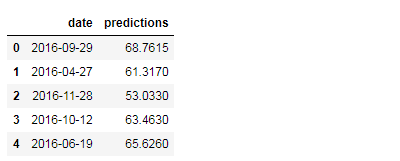
predictions_data=pd.DataFrame(data={'date':test_dates,
                                   'predictions':predictions})
predictions_data.head(5)                                                                     

作比较图：

plt.plot(ture_data['date'],ture_data['actual'],
        'b-',label='actual')
plt.plot(predictions_data['date'],predictions_data['predictions'],
        'ro',label='pedictions')
plt.xticks(rotation='60')
plt.legend()
plt.xlabel('Date')
plt.ylabel('Maximun temp')
plt.title('actual vs predict')

因为这里是对test_data进行的预测，不是对全部数据，所以展示的预测点是其中一部分。