梯度下降(code1.2)

理物迷

已于 2024-08-15 17:55:09 修改

阅读量688

点赞数 24

分类专栏：机器学习文章标签：机器学习算法

于 2024-08-15 17:52:25 首次发布

本文链接：https://blog.csdn.net/2303_78834656/article/details/141227113

版权

机器学习专栏收录该内容

6 篇文章 0 订阅

订阅专栏

梯度下降算法

代码课

现在，我们一起来编写梯度下降算法的代码。

考虑到更新公式：

$w=w-\alpha \frac{\partial J}{\partial w}$

$b=b-\alpha \frac{\partial J}{\partial b}$

函数需具备一下参数：

w_in，b_in，a

对于梯度，有以下方案可供选择：

请添加图片描述

于是乎，我们设置参数 gradient_function 用于计算梯度。

为了实时监控模型训练情况，很有必要间隔一段时间后输出当前拟合情况。我们在函数中写一段 log 输出代码，需设置 cost_function 参数，计算并反馈当前代价函数值。

对于停止更新条件的设计，我们有一下方案：
梯度下降终止条件
故还要给函数设置一个参数 iteration 控制迭代次数。

最终可设计以下算法流程图。

请添加图片描述

开始敲代码。

# import necessary modules.
from __future__ import annotations # annotation
import numpy as np # array
import pandas as pd # show datas.
import matplotlib.pyplot as plt # draw figures.
np.set_printoptions(precision=2) # set the display precision of numpy.

def gradient(x: ArrayLike, y: ArrayLike, w: float, b: float) -> tuple:
    # Use to calculate the gradient of squared error cost function in give point of (w, b)
    m = x.shape[0]
    dj_dw = 0
    dj_db = 0
    for i in range(0, m):
        err = w*x[i]+b-y[i]
        dj_dw += err*x[i]
        dj_db += err
    dj_dw = dj_dw/m
    dj_db = dj_db/m
    return (dj_dw, dj_db)

def squaredErrorCost(x: ArrayLike, y: ArrArrayLike, w: float, b: float):
    # Use to calculate the value of squared error cost function in give point of (w, b)
    m = x.shape[0]
    cost = 0
    for i in range(0, m):
        err = w*x[i]+b-y[i]
        cost += err**2
    cost = cost/(2*m)
    return cost

def gradientDescent(
    x: ArrayLike,
    y: ArrayLike,
    a: float,
    gradient: function,
    cost: function,
    iteration: int = 10000,
    w_in: float = 1,
    b_in: float = 0,
) -> tuple:
    # Use to operate the gradient descent to upgrade w, b
    w_init = w_in
    b_init = b_in
    cost_now = 0
    save_interval = np.ceil(iteration/10)
    for it in range(0, iteration):
        dj_dw, dj_db = gradient(x, y, w_init, b_init)
        w_init = w_init-a*dj_dw
        b_init = b_init-a*dj_db
        cost_now = cost(x, y, w_init, b_init)
        if it == 0 or it % save_interval == 0:
            print(f"iteration:{it}, cost:{cost_now:0.2e}")
    print(f"Final w:{w_init},b:{b_init},cost:{cost_now}")
    return (w_init, b_init)

# test example
x_emp = np.arange(0, 10)
y_emp = np.arange(0, 10)
a_emp = 1e-3
w_emp = 1
b_emp = 0

# test squareErrorCost().
squaredErrorCost(x_emp, y_emp, w_emp, b_emp) # np.float64(0.0)

# test gradient().
gradient(x_emp, y_emp, w_emp, b_emp) # (np.float64(0.0), np.float64(0.0))

# test gradientDescent.
gradientDescent(x_emp, y_emp, a_emp, gradient, squaredErrorCost, 10000, 1, 0) #  (np.float64(1.0), np.float64(0.0))

# import real data to learn. 
train_example = np.loadtxt(fname="../data/data1.txt", delimiter=",")
col_lable = ['size', 'floors', 'price']
df = pd.DataFrame(train_example, columns=col_lable) #

print(df) # The result is as follows

	size	floors	price
0	2104.0	3.0	399900.0
1	1600.0	3.0	329900.0
2	2400.0	3.0	369000.0
3	1416.0	2.0	232000.0
4	3000.0	4.0	539900.0
5	1985.0	4.0	299900.0
6	1534.0	3.0	314900.0
7	1427.0	3.0	198999.0
8	1380.0	3.0	212000.0
9	1494.0	3.0	242500.0
10	1940.0	4.0	239999.0
11	2000.0	3.0	347000.0
12	1890.0	3.0	329999.0
13	4478.0	5.0	699900.0
14	1268.0	3.0	259900.0
15	2300.0	4.0	449900.0
16	1320.0	2.0	299900.0
17	1236.0	3.0	199900.0
18	2609.0	4.0	499998.0
19	3031.0	4.0	599000.0
20	1767.0	3.0	252900.0
21	1888.0	2.0	255000.0
22	1604.0	3.0	242900.0
23	1962.0	4.0	259900.0
24	3890.0	3.0	573900.0
25	1100.0	3.0	249900.0
26	1458.0	3.0	464500.0
27	2526.0	3.0	469000.0
28	2200.0	3.0	475000.0
29	2637.0	3.0	299900.0
30	1839.0	2.0	349900.0
31	1000.0	1.0	169900.0
32	2040.0	4.0	314900.0
33	3137.0	3.0	579900.0
34	1811.0	4.0	285900.0
35	1437.0	3.0	249900.0
36	1239.0	3.0	229900.0
37	2132.0	4.0	345000.0
38	4215.0	4.0	549000.0
39	2162.0	4.0	287000.0
40	1664.0	2.0	368500.0
41	2238.0	3.0	329900.0
42	2567.0	4.0	314000.0
43	1200.0	3.0	299000.0
44	852.0	2.0	179900.0
45	1852.0	4.0	299900.0
46	1203.0	3.0	239500.0

# create input variable and target variable
x_train = train_example[:, 0] # x: size
y_train = train_example[:, 2] # y: price
a = 1e-8 # set learning rate

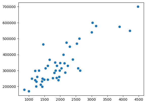
# see the distribution of (x, y), using matplotlib.pyplot.scatter. 
plt.scatter(x_train, y_train)

    # Python result, Not code!!!
    <matplotlib.collections.PathCollection at 0x777f1bfe3290>

png

# Run gradient descent
w, b = gradientDescent(x_train, y_train, a, gradient, squaredErrorCost, 10000, w_in=0, b_in=0) # The result is as follows

    # Python result, Not code!!!
    iteration:0, cost:5.99e+10
    iteration:1000, cost:2.40e+09
    iteration:2000, cost:2.40e+09
    iteration:3000, cost:2.40e+09
    iteration:4000, cost:2.40e+09
    iteration:5000, cost:2.40e+09
    iteration:6000, cost:2.40e+09
    iteration:7000, cost:2.40e+09
    iteration:8000, cost:2.40e+09
    iteration:9000, cost:2.40e+09
    Final w:165.38277501279427,b:1.0249605653820617,cost:2397855952.0764656

# Visualize it.
plt.scatter(x_train, y_train)
plt.plot(x_train, w*x_train+b, color='r')
plt.show()

    [<matplotlib.lines.Line2D at 0x777f1bdbcc90>]

png

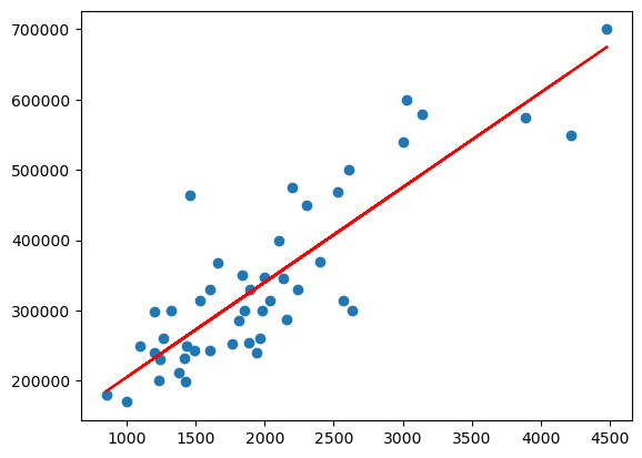
Perfect!

讨论

可以发现这里的学习率 a 十分的小，1e-8。事实上，我们无法提高 a 的值了，否则会导致梯度下降算法剧烈震荡，以至于不能收敛(convergent)。这是很恐怖的，会直接导致代价函数值不降低反升，最终溢出，具体在可视化(visualization)章节有具体的讲述。事实上，正常的学习率都不该这么小的，此处由于没有进行特征缩放(feature scaling)，我们只能容忍这么一个小的 a；
从数据集中可以看出，影响 price 的变量不止一个，要解决多变量的线性回归问题，需要借助"向量化"(vetorization)这一强大的工具；
我们发现最终 cost 趋于平稳，可不是 cost 达到了最小值。事实上，我们利用线性回归系数公式计算发现，J 还能取到更小的值。如下：

def regressionCoef(x: ArrayLike, y: ArrayLike):
    # Use to calculate the regression coefficients.
    m = x.shape[0] # raw of x
    x_bar = x.mean() # average of x
    y_bar = y.mean() # average of y
    sum_xiyi = 0
    sum_xixi = 0
    sum_xiyi = np.dot(x, y)
    sum_xixi = np.dot(x, x)
    # The regression coefficient fomulas
    w = (sum_xiyi-m*x_bar*y_bar)/(sum_xixi-m*x_bar*x_bar)
    b = y_bar-w*x_bar
    print(f"w:{w},b:{b}")
    return (w, b)

w, b = regressionCoef(x_train, y_train) # w:134.52528772024127,b:71270.49244872923

squaredErrorCost(x_train, y_train, w, b) # np.float64(2058132740.4330416)

cost 稳定只是显示的问题，“print(f"iteration:{it}, cost:{cost_now:0.2e}”)"。事实上，如果将显示位数提高，我们能发现 cost 在以一个非常慢的速率变小。之所以这么慢，是因为此时 $\frac{\partial J}{\partial w}$ $\frac{\partial J}{\partial b}$ 过小，w , b 更新缓慢。

4. 细心的人还发现，此时的 cost 仍然很大，比我们暴力枚举获得的 cost 还大，这足以说明影响造成 cost 过大的主要原因才不是 w,b 的选择。而是受模型结构的影响，模型本身的 cost 就很大。
5. 我们越来越发现可视化的重要意义。能辅助我们选择模型，验证拟合情况……。随着我们学习的深入，我们会发现更多的意义。

下节预告：

可视化

理物迷

关注

24
点赞
踩
20

收藏

觉得还不错? 一键收藏
0
评论
梯度下降(code1.2)

现在，我们一起来编写梯度下降算法的代码。ww−α∂w∂Jbb−α∂b∂J函数需具备一下参数：对于梯度，有以下方案可供选择：于是乎，我们设置参数 gradient_function 用于计算梯度。为了实时监控模型训练情况，很有必要间隔一段时间后输出当前拟合情况。我们在函数中写一段 log 输出代码，需设置 cost_function 参数，计算并反馈当前代价函数值。
复制链接

扫一扫

专栏目录