线性回归模型(code1.1)

代码课1.1(线性回归，穷举参数)

先导入有关模块

# import annotations
from __future__ import annotations
# import time to calculate the program running time
import time
# import numpy, using narray to store the data.
import numpy as np
# import matplotlib to draw figures
import matplotlib.pyplot as plt

定义 模型结构 与 损失函数
本质上就是用代码去描述一遍数学表达式

# create the model
def f(w: float, x: ArrayLike, b: float) -> ArrayLike:
    y_hat = np.array([])
    for i in x:
        p = w*i+b
        y_hat = np.append(y_hat, p)
    return y_hat

# create the cost function
def squaredErrorCost(y: ArrayLike, y_hat: ArrayLike) -> float:
    m = y.size
    err = y_hat - y
    cost = np.dot(err, err)
    cost = cost.sum()/(2*m)
    return cost

养成良好的习惯，写好函数后，编个简单的测试用例，进行检验。不然以后要 Debug 就不容易了。

# Simply verify the written function
x = np.array([1, 2, 3, 4])
y = np.array([2, 4, 6, 7])
y_hat = f(2, x, 0)
J = squaredErrorCost(y, y_hat)
print(f"The predictions {y_hat}, the cost {J}")

The predictions [2. 4. 6. 8.], the cost 0.125

导入数据集合，数据集可以去网上下载，也可以自己编写。

# import datas
data = np.loadtxt(fname="../data/data.txt", delimiter=',')
# create training examples
x = data[..., 0]
y = data[..., 2]

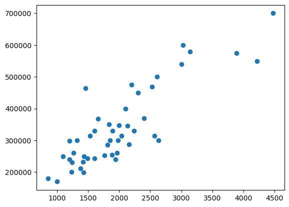
数据导入完毕后，将其可视化。经观察发现，数据确实存在一定的线性关系，可以用来训练线性回归模型。

数据可视化(data visualization) 是个非常重要的技能，它能辅助我们选择合适的模型，判断模型训练情况等。下期，我们将重点介绍这个。

plt.scatter(x, y)

<matplotlib.collections.PathCollection at 0x75d4050f8410>

​

​

准备工作完成之后，我们就可以通过一定的算法来训练模型了。由于我们现在只会穷举，就先将就着用吧，主要目的在于体验这个过程。以后，我们通过不断学习，逐步优化我们的训练代码。
基于现有的知识，寻找合适的解决方案，不失是一种智慧。
我们遇到的问题是：算力不够，时间有限，不可能枚举所有的 w,b。
解决方案：依照数据集，先给定一个合理的 w,b 范围。再依据训练得到的反馈，手动修正范围，逐步获得优化的 w,b。
操作：

1. 先从 (100,600) 中等间隔取 100 个数作为 w，从 (10000,20000) 中等间隔取 100 个数作为 b；
2. 运行后发现，b=10000；
3. 将 b 范围调整为 (0,10000) 继续尝试与调整；
4. 感觉 J 值合理，停止操作。
   以下给出 w (100,600)，b (0,10000) 时的情况

# Because we haven't learned gradient descent,
# we can only use exhaustion method first.
# Let's just have a try for fun.
start = time.time()
J_hist = []
for w in np.linspace(100, 600, 100):
    for b in np.linspace(0, 100000, 100):
        y_hat = f(w, x, b)
        J_hist.append((w, b, squaredErrorCost(y, y_hat)))
J_hist.sort(key=lambda x: x[2])
w = J_hist[0][0]
b = J_hist[0][1]
cost = J_hist[0][2]
end = time.time()
print(f"w:{w}, b:{b}, J:{cost}, running time:{end-start}")

w:135.35353535353534, b:69696.9696969697, J:2058348241.0833101, running time:2.1354281902313232

我们吃惊地发现，J 值竟然有 20 亿！不用害怕，由于我们的模型过于粗糙，今后学习了梯度下降，特征缩放，特征工程等后，我们会逐步把 J 压下去的。
你可能想增大等间隔取的参数个数，来获得更优模型，下面的代码，可以给我们带来一些思考。

start = time.time()
J_hist = []
for w in np.linspace(100, 600, 1000):
    for b in np.linspace(0, 100000, 100):
        y_hat = f(w, x, b)
        J_hist.append((w, b, squaredErrorCost(y, y_hat)))
J_hist.sort(key=lambda x: x[2])
w = J_hist[0][0]
b = J_hist[0][1]
cost = J_hist[0][2]
end = time.time()
print(f"w:{w}, b:{b}, J,:{cost}, running time:{end-start}")

w:134.53453453453454, b:71717.17171717172, J,:2058240962.6992188, running time:19.46424102783203

很明显，J 并没有减少多少，但运行时间却增加了 9 倍。
或许，并不是我们的 w,b 不合理，而是利用线性模型 J 值就小不了。但这不是说线性模型无能，今后通过对线性模型的包装，我们是能够将 J 值降到很小的。
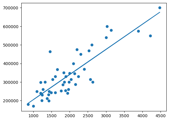
下面的图像现实，我么们的 w,b 取的并不差。

y_predit = f(w, x, b)
plt.scatter(x, y)
plt.plot(x, y_predit)
plt.show()

​

​

不过，为了获得最适合的 w,b 值，以及解决一些更复杂的 w,b 取值问题，我们有必要了解梯度下降算法。即使我们知道，对于今天的问题，就算用梯度下降算法，或许也无济于事。