机器学习学习笔记3-CSDN博客

本文链接：https://blog.csdn.net/2401_82787858/article/details/137961478

L5 回归建模

回顾

分类和回归的比较：

Classification

Datum i : feature vector $x^{(i)}=(x_1^{(i)},...,x_d^{(i)})^{\top}\in\mathbb{R}^{d}\\$ label $y^{(i)}\in\{-1,1\}$
Hypothesis h : $\mathbb{R}^d\to\{-1,+1\}$
Loss : 0-1 , asymmetric , NLL(负对数似然损失)
Example : linear classification

Regression

Datum i : feature vector $x^{(i)}=(x_1^{(i)},...,x_d^{(i)})^{\top}\in\mathbb{R}^{d}\\$ label $y^{(i)}\in\mathbb{R}$
Hypothesis h : $\mathbb{R}^d\to\mathbb{R}$
Loss : $L(g,a) = (g-a)^2$
Example : linear regression

Linear regression

Hypothesis : $h(x;\theta,\theta_0) = \theta^{\top}x+\theta_0$
Training error(平方损失）

$J(\theta,\theta_0)=\frac{1}{n}\sum_{i=1}^{n}L(h(x^{(i)};\theta,\theta_0),y(i))=\frac{1}{n}\sum_{i=1}^n(\theta^{\top}x^{(i)}+\theta_0-y(i))^2$

$\theta$ dimension agument

$J(\theta) = \frac{1}{n}\sum_{i=1}^{n}(\theta^{\top}x^{(i)}-y^{(i)})^2= \frac{1}{n}\sum_{i=1}^n((x^{(i)})^{\top}\theta-y^{(i)})^2\\ =\frac{1}{n}||\tilde{X}\theta-\tilde{Y}||^2=\frac{1}{n}(\tilde{X}\theta-\tilde{Y})^{\top}(\tilde{X}\theta-\tilde{Y})$

A Direct Solution

Goal : minimize $J(\theta) = \frac{1}{n}(\tilde{X}\theta-\tilde{Y})^{\top}(\tilde{X}\theta-\tilde{Y})$
Uniquely minimized at a point when gradient is zero
Gradient $\nabla_{\theta} J(\theta)\\$

$=\frac{2}{n}\tilde{X}^{\top}(\tilde{X}\theta-\tilde{Y}) \stackrel{set}{=}0\\ \Rightarrow \theta = (\tilde{X}^{\top}\tilde{X})^{-1}\tilde{X}^{\top}\tilde{Y}$

Matrix of second derivatives $\frac{2}{n}\tilde{X}^{\top}\tilde{X}$

Wrong in practice

超平面不唯一（数据线性相关）
噪声
$\theta$ 中各个值在零附近

Regularizing linear regression(正交化)

With square penalty : ridge regression

$J_{ridge}(\theta,\theta_0)=\frac{1}{n}\sum_{i=1}^n(\theta^{\top}x^{(i)}+\theta_0-y(i))^2+\lambda||\theta||^2$

Special case : with no offset

$J_{ridge}(\theta)=\frac{1}{n}(\tilde{X}\theta-\tilde{Y})^{\top}(\tilde{X}\theta-\tilde{Y})+\lambda||\theta||^2 =\frac{1}{n}||\tilde{X}\theta-\tilde{Y}||^2+\lambda||\theta||^2$

Min at : $\nabla_{\theta} J_{ridge}(\theta)=0$

$\\ \Rightarrow \theta = (\tilde{X}^{\top}\tilde{X}+n\lambda E)^{-1}\tilde{X}^{\top}\tilde{Y}$

Matrix of second derivatives $\tilde{X}^{\top}\tilde{X}+n\lambda E$

Gradient descent for linear regression

LR-Gradient-Descent $(\theta_{init},\theta_{0,init},\eta,T)$

Initialize $\theta^{(0)}=\theta_{init}$

Initialize $\theta_0^{(0)}=\theta_{0,init}$

for t = 1 to T

$\theta^{(t)}=\theta^{(t-1)}-\eta\{\frac{2}{n}\sum_{i=1}^n[\theta^{(t-1)\top}x^{(i)}+\theta_0^{(t-1)}-y^{(i)}]x^{(i)}+2\lambda\theta^{(t-1)}\}$

$\theta_0^{(t)}=\theta_0^{(t-1)}-\eta\{\frac{2}{n}\sum_{i=1}^n[\theta^{(t-1)\top}x^{(i)}+\theta_0^{(t-1)}-y^{(i)}]\}$

Return $\theta^{(t)},\theta_0^{(t)}$

Stochastic gradient descent 随机梯度下降

Stomachastic-Gradient-Descent $(\Theta_{init},\eta,T)$

Initialize $\Theta^{(0)}=\Theta_{init}$

for t = 1 to T

randomly select i from {1,...,n} (w.e.p)

$\Theta^{(t)}=\Theta^{(t-1)}-\eta(t)\nabla_{\Theta} f_i(\Theta^{(t-1)})$

Return $\Theta^{(t)}$

L6 神经网络 neutral nets

回顾

Linear classification with default features

Linear classification with polynomial features : $\phi(x)=[x_1,x_2,x_1^2,x_1x_2,x_2^2]^{\top}$

New Features : step functions

$\phi_1(x)=1\{\omega^{\top}x+\omega_0\geq0\}$
$\phi_2(x)=1\{\tilde\omega^{\top}x+\tilde\omega_0\geq0\}$
$\phi_3(x)=1\{\tilde\tilde\omega^{\top}x+\tilde\tilde\omega_0\geq0\}$

$z=\theta^{\top}\phi(x)+\theta_0\\ =\theta_{1}\phi_1(x)+\theta_{2}\phi_2(x)+\theta_{3}\phi_3(x)+\theta_0\\ =1\phi_1(x)+1\phi_2(x)+1\phi_3(x)+(-0.5)$

NN,some new notation

1st layer ,constructing the features :

Input x(a data point) : size $m^{(1)}\times1 (m^{(1)}=d)$
Output $A^{(1)}$ (vector of features) : size $n^{(1)}\times1$
The ith feature : $A_i^{(1)}=f^{(1)}(\omega_i^{(1)\top}x+\omega_0^{(1)})$
All the features at once:

$A^{(1)}=f^{(1)}(W^{(1)\top}x+W_0^{(1)})\\ W^{(1)}:m^{(1)}\times n^{(1)};W_0^{(1)}:n^{(1)}\times 1$

2nd layer ,assigning a label(or labels) :

Input (the features) : size $m^{(2)}\times1 (m^{(2)}=n^{(1)})$
Output $A^{(2)}$ (vector of labels) : size $n^{(2)}\times1$
The ith feature : $A_i^{(2)}=f^{(2)}(\omega_i^{(2)\top}A^{(1)}+\omega_0^{(2)})$
All :

$A^{(2)}=f^{(2)}(W^{(2)\top}A^{(1)}+W_0^{(2)})\\ W^{(2)}:m^{(2)}\times n^{(2)};W_0^{(2)}:n^{(2)}\times 1$

Whole thing : $A^{(2)}=NN(x;W,W_0)$

For one neuron/unit/node : $x_i\to\sum\to Z_i^{(1)}\to f^{(1)} \to A_i^{(1)}$

inputs

dot product

pre_activation

activation function

activation

Forward vs. backward

A feed-forward neural network : RNN

Different activation functions

do regression : $f^{(2)}(z)=z$

use NLL loss : $f^{(2)}(z)=\sigma(z)$

Need non-zero derivatives for (S)GD : Above & $f^{(1)}(z)\in\{\sigma(z),tanh(z),ReLU(z)\}$

Learning the parameters

目标函数： $J(W,W_0)= \frac{1}{n}\sum_{i=1}^nL(h(x^{(i)};W;W_0),y^{(i)})$

如果目标函数平滑且有唯一极值，(S)GD perform well !

import numpy as np
import matplotlib.pyplot as plt
from sklearn.datasets import load_digits
from sklearn.model_selection import  train_test_split
from sklearn.preprocessing import StandardScaler
from sklearn.neural_network import MLPClassifier
from sklearn.metrics import accuracy_score

# 加载手写数字识数据集
digits = load_digits()
X = digits.data
y = digits.target

# 数据标准化
scaler = StandardScaler()
X_scaled = scaler.fit_transform(X)

# 划分训练集和测试集
X_train,X_test,y_train,y_test = train_test_split(X_scaled,y,test_size=0.2,random_state=42)

# 构建神经网络模型
mlp = MLPClassifier(hidden_layer_sizes=(100,50),activation='relu',solver='adam',max_iter=500,random_state=42)

# 训练模型
history = mlp.fit(X_train,y_train)

# 预测并计算准确率
y_pred = mlp.predict(X_test)
accuracy = accuracy_score(y_test,y_pred)
print('Accuracy:',accuracy)

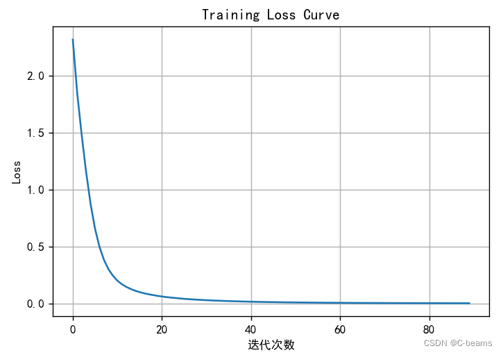
# 绘制训练过程中的损失曲线
plt.rcParams['font.sans-serif']=['SimHei']
plt.rcParams['axes.unicode_minus'] = False
plt.figure(figsize=(10,6))
plt.plot(history.loss_curve_)
plt.title('Training Loss Curve')
plt.xlabel('迭代次数')
plt.ylabel('Loss')
plt.grid(True)
plt.show()

Accuracy: 0.9805555555555555