机器学习学习笔记2

最新推荐文章于 2024-07-25 18:25:30 发布

C-beams

最新推荐文章于 2024-07-25 18:25:30 发布

阅读量689

点赞数 15

分类专栏：机器学习学习笔记文章标签：机器学习学习笔记

本文链接：https://blog.csdn.net/2401_82787858/article/details/137854259

版权

机器学习学习笔记专栏收录该内容

6 篇文章 0 订阅

订阅专栏

L3 Feature 特征

Encode data

将特征转化为实数

什么是特征？任何可获取的数据（除了label标签）

old features: $x$ new features: $\phi (x)$

Encode categorical data

Idea：将每个类别转化为独一无二的二进制数(通常不用)

e.g.

	$\phi _d$	$\phi_{d+1}$	$\phi_{d+2}$
nurse	0	0	0
admin	0	0	1
pharmacisst	0	1	0
doctor	0	1	1
social worker	1	0	1

Idea：将每个类别转化为唯一的 0-1 数字（“one-hot encoding”）（使用于各类别无明显相关性）

e.g.

	$\phi _d$	$\phi_{d+1}$	$\phi_{d+2}$	$\phi_{d+3}$	$\phi_{d+4}$
nurse	1	0	0	0	0
admin	0	1	0	0	0
pharmacisst	0	0	1	0	0
doctor	0	0	0	1	0
social worker	0	0	0	0	1

Idea：因子编码（单个数据包含多个因素）

e.g.

	$\phi _d$	$\phi_{d+1}$
pain	1	0
pain&blockers	1	1
blockers	0	1
no medications	0	0

Encode ordinal(序数) data

Idea：Unary/thermometer code 温度计编码（各个值区别较大）

e.g.Likert scale 李克特量表

Strongly disagree	Disagree	Neutral	Agree	Strongly agree
1,0,0,0,0	1,1,0,0,0	1,1,1,0,0	1,1,1,1,0	1,1,1,1,1

Encode numerical data

Idea：标准化

for $d_{th}$ feature: $\phi_{d}^{(k)}=\frac{x_{d}^{(k)}-mean_d}{stddev_d}$

Nonlinear boundaries 不可线性分割的数据

Idea：用k次泰勒多项式逼近到一个平滑函数

order(k)	terms when d=1	terms for general d
0	$[1]$	$[1]$
1	$[1,x_1]$	$[1,x_1,...,x_d]$
2	$[1,x_1,x_1^{2}]$	$[1,x_1,...,x_d\\ x_1^2,x_1x_2,...,x_{d-1}x_d,x_d^2]$
3	$[1,x_1,x_1^2,x_1^3]$	$[1,x_1,...,x_d\\ x_1^2,x_1x_2,...,x_{d-1}x_d,x_d^2\\ x_1^3,x_1^2x_2,x_1x_2x_3,...,x_d^3]$

Evaluation of a learning algorithm

Idea:使用全部数据训练然后求出训练误差

Idea:保留一些数据用来测试

More training data:closer to training on full data
More testing data:less noisy estimate of performance
Only one classifier might not be representative
Good idea to shuffle order of data

伪代码如下：

Cross-validate $(D_n,k)$ #交叉验证

Divide $D_n$ into k chunks $D_{n,1},...,D_{n,k}$ (for roughly equal size)

for i = 1 to k

train $h_i$ on $D_n \setminus D_{n,i}$ (i.e. except chunk i)

compute "test" error $\varepsilon (h_i,D_{n,i})\ of \ hi \ on\ D_{n,i}$

Return $\frac{1}{k}\sum_{i=1}^k\varepsilon (h_i,D_{n,i})$

代码如下：

import matplotlib.pyplot as plt
from sklearn import neighbors
import numpy as np
import pandas as pd
from sklearn import model_selection
df1 = pd.read_csv(r'iris.csv')
print(df1.head())#输出前五行
predictors = df1.columns[:-1]
x_train,x_test,y_train,y_test=model_selection.train_test_split(
    df1[predictors],df1.Species,
    test_size=0.5,
    random_state = 1234
)
print(np.ceil(np.log2(df1.shape[0])))
#设置待测试的不同K值
K = np.arange(1,np.ceil(np.log2(df1.shape[0])))
print(np.arange(1,np.ceil(np.log2(df1.shape[0]))))
#设置空列表，用于储存平均准确率
accuracy = []
# 使用五重交叉验证的方法
for k in K:
    cv_result = model_selection.cross_val_score \
        (neighbors.KNeighborsClassifier(n_neighbors=int(k),
                                        weights='distance'),
         x_train, y_train, cv=5, scoring='accuracy')
    accuracy.append(cv_result.mean())

# 从K个平均准确率中挑选出最大值做对应的目标
arg_max = np.array(accuracy).argmax()
#中文负号正常显示
plt.rcParams['font.sans-serif']=['SimHei']
plt.rcParams['axes.unicode_minus'] = False
#绘制不同k值与准确率之间的折线图
plt.plot(K,accuracy)
plt.scatter(K,accuracy)
plt.text(K[arg_max],accuracy[arg_max],'最佳K值为%s'%int(K[arg_max]))
plt.show()

L4 Logistic regression 逻辑回归/对数几率回归

回顾：感知器难以处理不可线性分割的数据

sigmoid/logistic function

$\sigma(z)=\frac{1}{1+exp(-z)}$

$g(x)=\frac{1}{1+exp\{-(\theta^{\top}x+\theta_0)\}}$

Linear logistic classification

如何得到一个一个分类器 $learn \ \theta,\theta_0$

Probability(data)

$=\prod _{i=1}^nProbability(data \ point\ i)\\ =\prod_{i=1}^n \begin{cases}g^{(i)}\ if\ y^{(i)}=+1\\(1-g^{(i)})else\end{cases}\\ =\prod_{i=1}^n(g^{(i)})^{1\ \{y_i=+1\}}(1-g^{(i)})^{1\{y_i\neq -1\}}$

Loss(data) = -(1/n)*log probability(data)

$=\frac{1}{n}\sum_{i=1}^n-(1\{y_i=+1\}logg^{(i)}+1\{y_i\neq+1\}log(1-g^{(i)}))$

Negative log likelihood loss:

$-L_{nll}(g,a) = (1\{a=+1\}logg+1\{a\neq+1\}log(1-g))$

learn $\theta,\theta_0$ ( i.e.to minimize average loss):

$J_{lr}(\Theta )=J_{lr}(\theta,\theta_0)=\frac{1}{n}\sum_{i=1}^nL_{nll}(\sigma(\theta^{\top}x^{(i)}+\theta_0),y^{(i)})$

Gradient descent 梯度下降

Gradient : $\nabla_{\Theta}f=\nabla_{\Theta}f=[\frac{\partial f}{\partial \Theta_1},...,\frac{\partial f}{\partial \Theta_1}]^{\top}$

伪代码如下：

Gradinent-Descent $(\Theta_{init},\eta,f,\nabla_\Theta f,\epsilon )$

Initialize $\Theta^{(0)}=\Theta_{init}$

Initialize $t = 0$

repeat

t = t + 1

$\Theta^{(t)}=\Theta^{(t-1)}-\eta\nabla_\Theta f(\Theta^{(t-1)})$

until $|f(\Theta^{(t)})-f(\Theta^{(t-1)})|<\epsilon$

Return $\Theta^{(t)}$

其他可能的停止条件：

达到最大迭代次数T
$|\Theta^{(t)}-\Theta^{(t-1)}|<\epsilon$
$||\nabla_{\Theta}f(\Theta^{(t)})||<\epsilon$

Logistic regression learning algorithm

LR-Gradient-Descent $(\theta_{init},\theta_{0,init},\eta,\epsilon )$

Initialize $\theta^{(0)}=\theta_{init}$

Initialize $\theta_0^{(0)}=\theta_{0,init}$

Initialize $t = 0$

repeat

t = t + 1

$\theta^{(t)}=\theta^{(t-1)}-\eta\{ \frac{1}{n}\sum_{i=1}^n[\sigma(\theta^{(t-1)\top}x^{(i)}+\theta_0^{(t-1)})-y^{(i)}]x^{(i)}+\lambda\theta^{(t-1)} \}$

$\theta_0^{(t)}=\theta_0^{(t-1)}-\eta\{ \frac{1}{n}\sum_{i=1}^n[\sigma(\theta^{(t-1)\top}x^{(i)}+\theta_0^{(t-1)})-y^{(i)}] \}$

until $|J_{lr}(\theta^{(t)},\theta_0^{(t)})-J_{lr}(\theta^{(t-1)},\theta_0^{(t-1)})|<\epsilon$

Return $\theta^{(t)},\theta_0^{(t)}$

import numpy as np
import pandas as pd
import matplotlib.pyplot as plt
from sklearn.datasets import load_iris
from sklearn.model_selection import train_test_split
from sklearn.linear_model import  LogisticRegression
from sklearn.metrics import  accuracy_score
from matplotlib.colors import ListedColormap

iris = load_iris()
X = iris.data[:,:2] # 可视化前两个特征
y = iris.target

# 划分训练集和测试集
X_train,X_test,y_train,y_test = train_test_split(X,y,test_size=0.2,random_state=42)

# 训练逻辑回归模型
lr = LogisticRegression()
lr.fit(X_train,y_train)

# 在测试及上进行预测
y_pred = lr.predict(X_test)

# 计算准确率
accuracy = accuracy_score(y_test,y_pred)
print('Accuracy:',accuracy)

# 绘制决策边界
x_min,x_max = X[:,0].min() - 0.5,X[:,0].max() + 0.5
y_min,y_max = X[:,1].min() - 0.5,X[:,1].max() + 0.5
xx,yy = np.meshgrid(np.arange(x_min,x_max,0.01),np.arange(y_min,y_max,0.01))
Z = lr.predict(np.c_[xx.ravel(),yy.ravel()])
Z = Z.reshape(xx.shape)

# 绘制结果
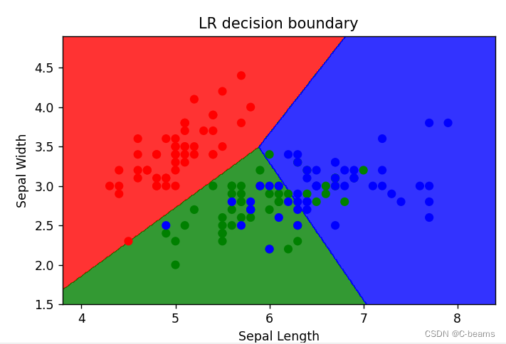
plt.figure(figsize=(10,6))
plt.contourf(xx,yy,Z,alpha=0.8,cmap=ListedColormap(('red','green','blue')))
plt.scatter(X[:,0],X[:,1],c=y,cmap=ListedColormap(('red','green','blue')))
plt.xlabel('Sepal Length')
plt.ylabel('Sepal Width')
plt.title('LR decision boundary')
plt.show()

输出结果：

Accuracy: 0.9