


L11 决策树与随机森林
Classfication tree
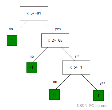
internal node : 1) dimension index j ;split value s ; 2) two child nodes : internal or leaf
leaf node : label
features: = [date,age,height,weight,sinus tachycardia?,min systolic bp]
labels y : 1:hight risk ; -1: low risk
Regression tree
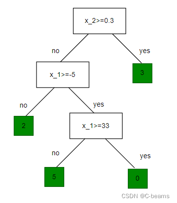
features: = [temperature(deg C),precipation(cm/hr)]
labels y : km run
- Tree defines an axis-aligned "partition" of the feature space
Decision tree
Recall : familiar pattern
- Choose how to predict label(given features & parameters))
- Choose a loss(between guess & actual label)
- Choose parameters by trying to minimize the training loss
Parameters here:
- For each internal node: split dimension , split value , child nodes
- For each leaf node : label
- Note : parameters here don't have a fixed dimension
- Can't apply (S)GD
- We'll develop a heuristic :1) build , 2) prune
Building a decision tree
- Regression tree with squared error loss
BuildTree(I,k)
if
set
return Leaf( label = )
else
for each split dim j & value s
Set
Set
Set
Set
Set
Set
return Node(
Regularize , prune and Ensembling
- "Cost complexity" of a tree T
- Pruning
- For each
, choose
by pruning subtrees until it's not worthwhile
- Choose a final tree by cross validation
- For each
- Using multiple machine learning predictors to make one(ideally way-better) predictor
Bagging
- One of multiple ways to make and use an ensemble
- Bagging = Bootstrap aggregating
- Training data
- For b = 1, ..., B
- Draw a new "data set"
of size n by sampling with replacement from
- Train a predictor
on
- For regression : the predictor
- Classification : predictor at a point is class with highest vote count at that point
- Draw a new "data set"
- Training data
Random forests
- Bagging + decision trees + extra randomness
- Random forest
- For b = 1, ..., B
- Draw a new "data set"
- Build a tree on
- Select m features uniformly at random,with out repacement,from the d features
- Pick the best split dimension and split value among the m features
- Build two children
- Draw a new "data set"
- Return: average for regression; vote for classification
- For b = 1, ..., B
import numpy as np
import matplotlib.pyplot as plt
from sklearn.datasets import load_iris
from sklearn.model_selection import train_test_split
from sklearn.ensemble import RandomForestClassifier
from sklearn.metrics import accuracy_score
from matplotlib.colors import ListedColormap

# 加载鸢尾花数据集
iris = load_iris()
X = iris.data[:,[2,3]] # 取特征的后两个维度
y = iris.target

# 划分训练集和测试集
X_train,X_test,y_train,y_test = train_test_split(X,y,test_size=0.3,random_state=42)

# 构建随机森林模型
rf_clf = RandomForestClassifier(n_estimators=100,random_state=42)
rf_clf.fit(X_train,y_train)

# 在测试集上预测
y_pred = rf_clf.predict(X_test)

# 计算模型准确率
accuracy = accuracy_score(y_test,y_pred)
print("Acuracy:",accuracy)

# 可视化决策边界
def plot_decision_regions(X,y,classifier,test_idx=None,resolution=0.2):
    markers = ('s','x','o','^','v')
    colors = ('red','blue','lightgreen','gray','cyan')
    cmap = ListedColormap(colors[:len(np.unique(y))])

    x1_min,x1_max = X[:,0].min()-1,X[:,0].max()+1
    x2_min, x2_max = X[:, 1].min() - 1, X[:, 1].max() + 1
    xx1,xx2 = np.meshgrid(np.arange(x1_min,x1_max,resolution),np.arange(x2_min,x2_max,resolution))
    Z = classifier.predict(np.array([xx1.ravel(),xx2.ravel()]).T)
    Z = Z.reshape(xx1.shape)
    plt.contourf(xx1,xx2,Z,alpha=0.5,cmap=cmap)
    plt.xlim(xx1.min(),xx1.max())
    plt.ylim(xx2.min(), xx2.max())

    for idx,cl in enumerate(np.unique(y)):
        plt.scatter(x=X[y==cl,0],y=X[y==cl,1],alpha=0.8,c=[cmap(idx)],marker=markers[idx],label=cl)
    if test_idx:
        X_test,y_test = X[test_idx,:],y[test_idx]
        plt.scatter(X_test[:,0],X_test[:,1],c='',edgecolors='black',alpha=1.0,linewidths=1,marker='o',s=100,label='Test Set')

plot_decision_regions(X_train,y_train,classifier=rf_clf)
plt.title('Random Forest Classifier - Decision Boundary(Training Set)')
plt.xlabel('Petal Length(cm)')
plt.ylabel('Petal Width (cm')
plt.legend(loc='upper left')
plt.show()
Acuracy: 1.0

L12 聚类算法
Food distribution placement
- Where should I have my k food trucks park?
- Want to minnimize the loss of people we serve.
- Inputs : person i location
- Outputs : truck j location
- Index of truck where people i walks :
- Loss if i walk to Truck j :
- Loss across all people :
a.k.a k-means objective
k-means algorithm
k-means
Init
for t = 1 to
for i = 1 to n
for j = 1 to k
if
break
return
Compare to classification
- 我们并没有使用任何标签数据
可以替换并且能得到相同的聚类簇k
- 输出仅仅只是数据的划分
- 我们根据数据间的相似性将他们分类
- 一个无监督学习的例子:没有标签数据,we're finding a pattern
Initialization
- If enough big
, it will converge
- The initialization can make a big difference
- Some options : random restarts
Effect of k and choosing k
- Different k will give us different results
- Larger k and smaller Loss
- Sometimes we know k
- Sometimes we'd like to choose/learn k
- How to choose k depends on what you'd like to do
import matplotlib.pyplot as plt
from sklearn.datasets import load_iris
from sklearn.cluster import KMeans
from sklearn.decomposition import PCA
from sklearn.preprocessing import StandardScaler

# 加载鸢尾花数据集
iris = load_iris()
X = iris.data
y = iris.target

#特征标准化
scaler = StandardScaler()
X_scaled = scaler.fit_transform(X)

# 使用PCA进行降维
pca = PCA(n_components=2)
X_pca = pca.fit_transform(X_scaled)

# 构建k均值聚类模型
kmeans = KMeans(n_clusters=3,random_state=42)
kmeans.fit(X_scaled)

# 获取聚类中心和预测类别
cluster_centers = kmeans.cluster_centers_
y_pred = kmeans.labels_

# 可视化聚类效果
plt.figure(figsize = (10,8))

# 绘制原始数据的散点图
plt.subplot(2,1,1)
plt.scatter(X_pca[:,0],X_pca[:,1],c=y,cmap='viridis',s=50,alpha=0.8)
plt.title('Original Data')
plt.xlabel('Principal Component 1')
plt.ylabel('Principal Component 2')

# 绘制聚类结果的散点图
plt.subplot(2,1,2)
plt.scatter(X_pca[:,0],X_pca[:,1],c=y_pred,cmap='viridis',s=50,alpha=0.8)
plt.scatter(cluster_centers[:,0],cluster_centers[:,1],c='red',marker='x',s=200,label='Cluster Centers')
plt.title('K-Means Clustering')
plt.xlabel('Principal Component 1')
plt.ylabel('Principal Component 2')
plt.legend()

plt.tight_layout()
plt.show()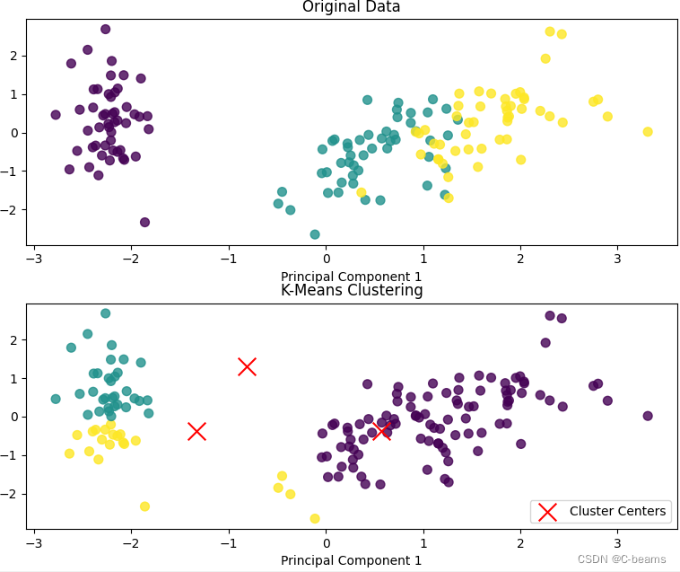


 8万+
8万+

 被折叠的 条评论
为什么被折叠?
被折叠的 条评论
为什么被折叠?
 到【灌水乐园】发言


